1. Genes, Proteins, Databases, Genome annotation

– Rens Holmer, Anne Kupczok, Tomer Sardjoe

Biological background

A large part of bioinformatics deals with the analysis of biological sequences. These sequences originate from organic macromolecules that play important roles in cells. In the first section of this chapter, we describe these macromolecules, their sequences, and the biological processes involved in generating their active structures and maintaining these.

As such, this section provides important background material for the entire course. Depending on your background, parts of this section might seem redundant, in which case this section can function as a refresher. Later chapters assume you are familiar with this section.

---

Nucleic acids

Deoxyribonucleic acid (DNA) carries the genetic information of organisms. Ribonucleic acid (RNA) is involved in the protein expression and is also the genetic material of some viruses. Thus, these molecules are highly important as the basis of life on Earth. The genome denotes the cell’s entire genetic content and genomics is the study of genomes.

DNA and RNA are comprised of monomers called nucleotides, which are comprised of three components (Fig. 1.1):

• A pentose sugar, where carbon residues are numbered 1’ to 5’ (read 1’ as “one prime”). The type of pentose distinguishes RNA and DNA: the sugar is deoxyribose in DNA and ribose in RNA. They are similar in structure, but deoxyribose has an H instead of an OH at the 2′ position.

• A phosphate group that is attached to the 5’ position of the sugar.

• A base that is attached to the 1’ position of the sugar.

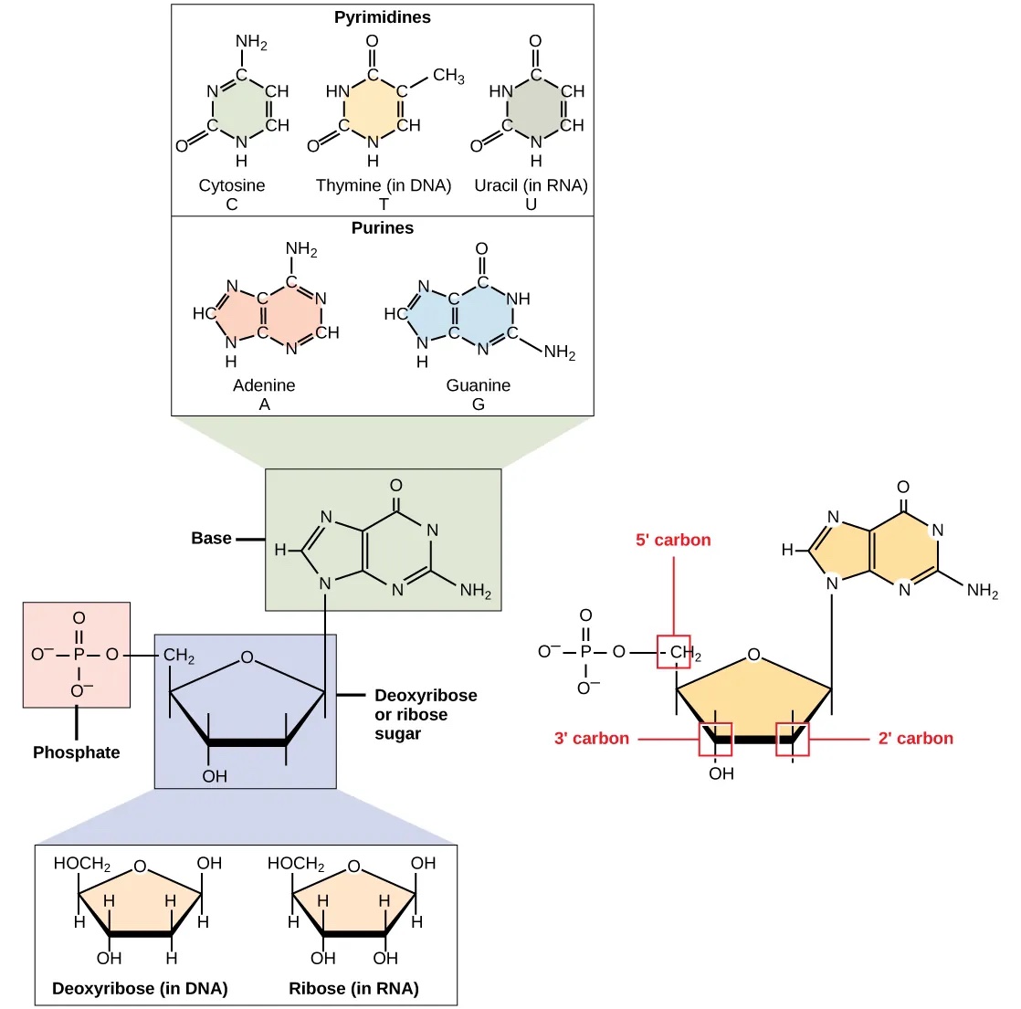
Fig. 1.1 The components of a nucleotide. Credits: CC BY 4.0 [Clark et al., 2018].

The bases can be divided into two categories: purines (with a double ring structure) and pyrimidines (with a single ring structure) (Fig. 1.1). DNA contains A, T, C, and G; whereas RNA contains A, U, C, and G.

Important

Nucleotides are central molecules in all life. You do not need to remember the exact chemical structure, but you need to know the difference between DNA and RNA, the different bases and their category (purines or pyrimidines).

---

The DNA double helix

The DNA molecule is a polymer of deoxyribonucleotides and forms a right-handed double helix. The sugar and phosphate are on the outside forming the helix’s backbone and the bases are stacked in the interior and bind each other by hydrogen bonds. Thereby A pairs with T via two hydrogen bonds and C pairs with G via three hydrogen bonds, they are complementary bases. These pairings are also called Watson-Crick base-pairing, named after the discoverers of DNA.

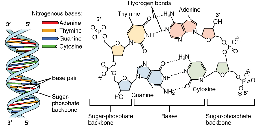
Fig. 1.2 The DNA structure. Credits: CC BY 3.0 [OpenStax College, 2013].

The two strands of the helix run in opposite directions, also called anti-parallel, i.e., one goes from 5’ to 3’ and the other from 3’ to 5’ (Fig. 1.2). The nucleotide sequence is typically written in 5’ to 3’ direction. Due to the complementarity, the base sequence of a strand can be deduced from the base sequence from the other strand. This is called the reverse complement. For example, the reverse complement of AAGT is ACTT, where both strands are given in 5’ to 3’ direction.

---

DNA replication

As the two DNA strands are only connected via hydrogen bonds, they can be separated relatively easily, for example during DNA replication (Fig. 1.3). The separated strands each serve as a template on which a new complementary strand is synthesized by the enzyme DNA polymerase in 5’ to 3’ direction. This mode of replication is called semiconservative.

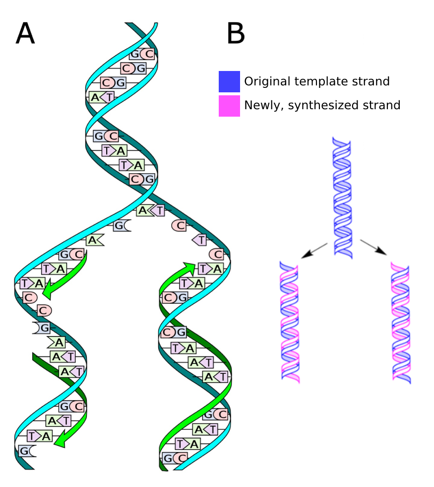
Fig. 1.3 A) The process of DNA replication. Credits: CC0 1.0 [Ball, 2013]. B) Semiconservative DNA replication, where the two copies each contain one original strand and one new strand. Credits: CC0 1.0 modified from [Koch, 2009].

The error rate of DNA replication is remarkably low, about one erroneous base in 10⁹ bases. This property preserves the genetic information during cell division, and also over generations. It also leads to mutations over evolutionary time (Fig. 1.4), as we will see later (Substitutions).

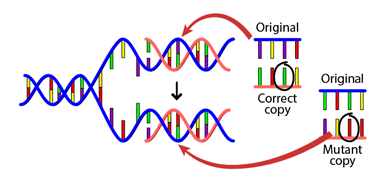
Fig. 1.4 A DNA mutation that occurs during replication. Credits: BY-NC-SA 4.0 [UC Museum of Paleontology, 2020].

---

RNA, transcription, and splicing

During transcription, RNA polymerase reads the template strand (also called noncoding strand) in the 3’ to 5’ direction (Fig. 1.5). This produces an RNA molecule from 5’ to 3’, which is a copy of the coding strand. During transcription thymine is replaced by uracil. In contrast to DNA, RNA does not form a stable double helix. RNA is mainly single stranded, but most RNAs show intramolecular base pairing between complementary bases.

There are four major types of RNA:

• Messenger RNA (mRNA): RNA molecules that will later be translated into proteins and therefore serve as a ‘messenger’ in protein production.

• Ribosomal RNA (rRNA): the primary component of ribosomes (the ‘powerplants’ of a cell).

• Transfer RNA (tRNA): functions as ‘adapter molecule’ that serve as the physical link between mRNA and the amino acid sequence of a protein during translation.

• MicroRNA (miRNA): non-coding RNA molecules of 21-23 nucleotides involved in RNA silencing and post-transcriptional regulation of gene expression.

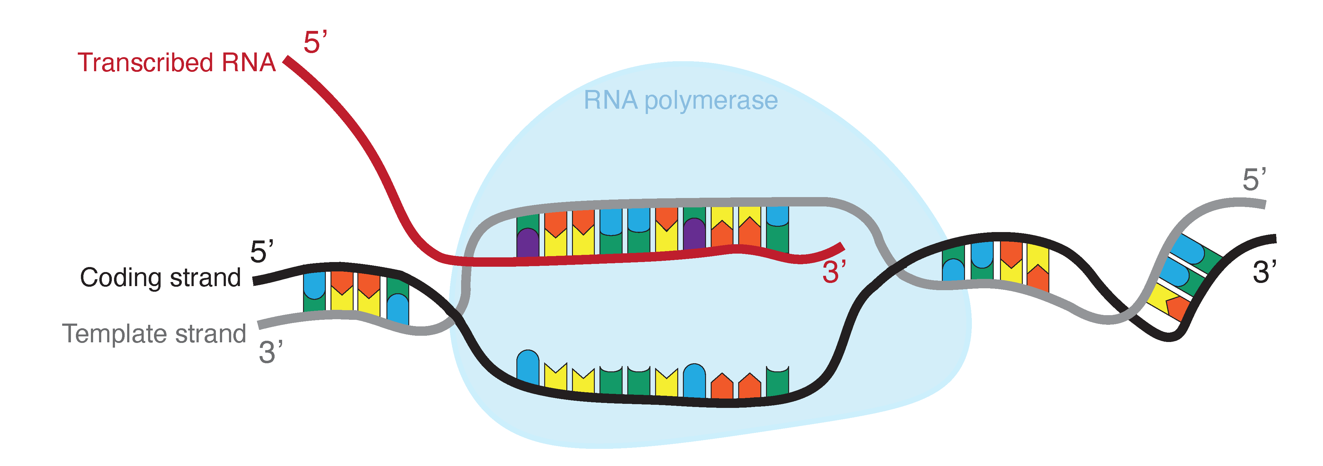
Fig. 1.5 RNA is produced by transcribing DNA: as such, it is a direct copy of the information contained in the DNA. Where DNA contains thymine (T, indicated in blue), RNA contains uracil (U, indicated in purple). Credits: CC BY-NC 4.0 [Ridder et al., 2024].

In eukaryotes, precursor mRNA molecules undergo splicing. During RNA splicing, the spliceosome protein complex removes introns: specific non-coding parts of an mRNA molecule that are not used during translation (Fig. 1.6), to create mature mRNA. Most introns are characterized by a GU and AG dinucleotide motif in the 5’ and 3’ end respectively.

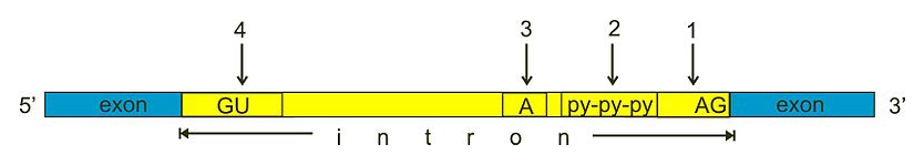
Fig. 1.6 During splicing, introns are removed from precursor mRNA moleculus to create mature mRNA. Most introns contain several canonical elements that help in recognition by the spliceosome and in creating a specific secondary structure of the intronic RNA that facilitates removal: (1) 3’ splice site, (2) poly pyrimidine tract, (3) branch site, (4) 5’ splice site’. Credits: CC0 1.0 [miguelferig, 2011].

---

Translation

During protein translation, ribosomes synthesize polypeptides from messenger RNA (mRNA) (Fig. 1.7). During this process tRNAs decode the information on the RNA into amino acids, where a codon consisting of three nucleotides encodes the information for one amino acid.

Fig. 1.7 The translation process, where ribosomes with tRNA molecules “read” codons on the mRNA using anticodons, which then get translated into their corresponding amino acids. These amino acids are linked together by peptide bonds to form a polypeptide chain. Credits: CC BY-NC 4.0 [Ridder et al., 2024].

See also

The details of transcription and translation differ between prokaryotes and eukaryotes. You can look up Chapters 15 and 16 of Biology 2e to learn more.

The genetic code

The genetic code shows the correspondence between codons and amino acids (Fig. 1.8). Since 64 possible codons code for 20 different amino acids, the genetic code is degenerate, i.e., most amino acids are specified by more than one codon. Thus, the codons encoding one particular amino acid may differ in one or two of their positions. You can notice in Fig. 1.8 that the third codon position often differs between codons for the same amino acid. As a result of the code degeneracy, the protein sequence can be deduced from the DNA or RNA sequence but not vice versa.

There are three codons that do not encode for an amino acid, but instead signal the end of the protein sequence, called stop codons. Furthermore, translation generally starts with the start codon AUG encoding methionine. More information of how protein information is encoded in genomes can be found in the section on genome annotation.

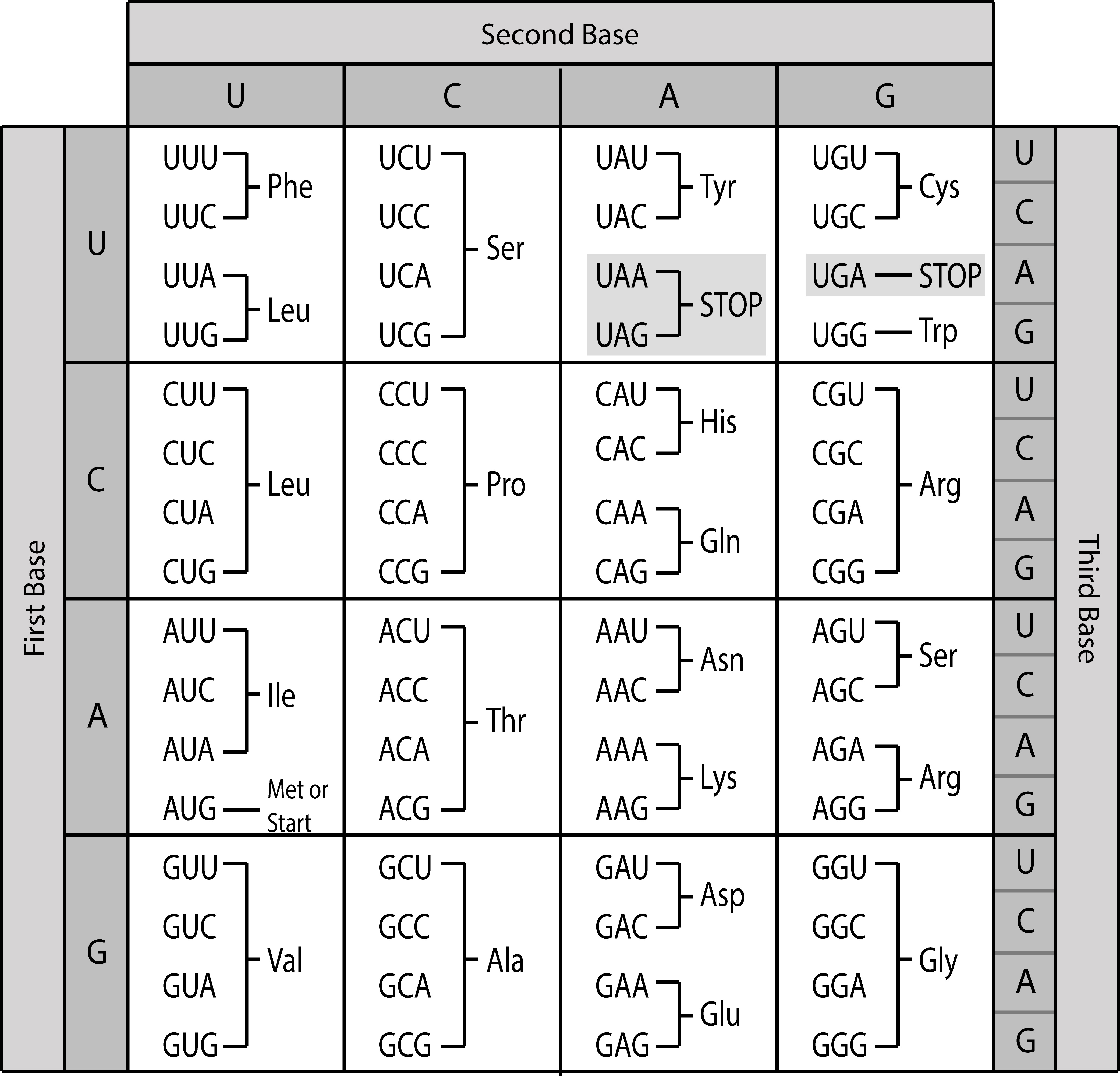
Fig. 1.8 The universal genetic code. Note that exceptions to this code exist, for example the vertebrate mitochondrial code. Credits: CC BY 4.0 [Greenwood, 2018].

Important

The universal genetic code is very important to understand how information flows from genes to proteins. Nevertheless, you do not need to recall it, but can always look it up. When needed, it will also be provided in the exam.

The central dogma of molecular biology

According to the central dogma of molecular biology, the flow of genetic information is essentially in one direction: from DNA via RNA to proteins (Fig. 1.9). Nevertheless, there are also genes that do not code for proteins, but where functional RNA is the end product. Furthermore, mobile genetic elements and viruses can encode reverse transcriptases (which can synthesize DNA from an RNA template) or RNA dependent RNA polymerases (which can replicate RNA).

Fig. 1.9 The central dogma of molecular biology. Credits: CC0 1.0 modified from [Squidonius, 2008].

Proteins

Proteins are large, complex macromolecules that play many important roles in the body. They are critical to most of the work done by cells and are required for the structure, function and regulation of the body’s tissues and organs. The basic building blocks of proteins are amino acids.

---

Amino acids

An amino acid contains a central carbon atom (called α-carbon, or C_α) (Fig. 1.10). The α-carbon is bound to an amino group (NH₂), a carboxyl group (COOH), and a hydrogen atom. In addition, each amino acid has a specific residue ® group.

Fig. 1.10 The structure of an amino acid. Four elements are connected to the α-carbon: an amino group, a hydrogen atom, a carboxyl group, and a side chain (R group). Credits: CC BY 4.0 [Clark et al., 2018].

Important

Amino acids differ in their chemical properties, which are determined by their R groups. It is important to know (by heart) the amino acids, their one-letter and three-letter abbreviation, and their fundamental properties as given in the table.

Amino acid	Three-letter code	One-letter code	Property
Arginine	Arg	R	Positively charged
Histidine	His	H	Positively charged
Lysine	Lys	K	Positively charged
Aspartic acid	Asp	D	Negatively charged
Glutamic acid	Glu	E	Negatively charged
Serine	Ser	S	Polar uncharged
Threonine	Thr	T	Polar uncharged
Asparagine	Asn	N	Polar uncharged
Glutamine	Gln	Q	Polar uncharged
Alanine	Ala	A	Hydrophobic
Valine	Val	V	Hydrophobic
Isoleucine	Ile	I	Hydrophobic
Leucine	Leu	L	Hydrophobic
Methionine	Met	M	Hydrophobic
Phenylalanine	Phe	F	Hydrophobic and aromatic
Tyrosine	Tyr	Y	Hydrophobic and aromatic
Trypotophan	Trp	W	Hydrophobic and aromatic
Glycine	Gly	G	Special (only H as side chain)
Proline	Pro	P	Special (side chain bound to backbone nitrogen)
Cysteine	Cys	C	Special (forms disulfide bonds)

Some amino acids have non-polar side chains, and these are generally hydrophobic, i.e., water molecules cannot form hydrogen bonds with these molecules. Thus, they can often be found in the interior of proteins together with other hydrophobic amino acids. Aromatic amino acids contain aromatic rings, and often stabilize folded protein structures.

In contrast, the charged and the polar amino acids are hydrophilic, i.e., water molecules can form hydrogen bonds with these molecules. They can often be found on the surface of proteins or in the interior, when they can interact with another oppositely charged amino acid. Positively charged amino acids, are also called basic amino acids and negatively charged amino acids are also called acidic amino acids.

Although amino acids can be classified into these groups based on their properties, some amino acids stand out. The smallest amino acid is glycine, which provides great flexibility due to its small size. In contrast, proline is an amino acid, where the side chain is bonded to the backbone nitrogen atom, which makes it very rigid.

---

Protein structure

A protein is made up of one or more long, folded chains of amino acids (each called a polypeptide). The 3D structure of a protein is also called its conformation. The protein conformation is described on four levels - primary to quaternary structure (Fig. 1.11).

Fig. 1.11 The four levels of protein structure. Credits: CC0 1.0 [LadyofHats, 2008].

The structure of a protein is critical for its function. For example, in an enzyme, the active site must be in the correct structure to be able to bind the substrate. Other proteins might bind proteins (and influence their activity) or bind DNA (and regulate gene expression). Additionally, some proteins are secreted from the cell or might function within the cell membrane. Finally, proteins are often modified after protein synthesis (see Translation), called post-translational modification. These modifications can be important for protein function.

---

Primary structure

In a protein, amino acids are connected by covalent bonds, called peptide bonds. A peptide bond connects one amino acid’s carobxyl group and the next amino acid’s amino group (Fig. 1.12). The sequence of amino acids linked by peptide bonds is called the primary structure. The protein sequence is determined by the gene sequence encoding the protein. The continuous chain of atoms along the protein is also called the backbone, it consists of the three backbone atoms (nitrogen, C_α, carbon).

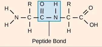
Fig. 1.12 A peptide bond connecting two amino acids. Credits: CC BY 4.0 [Clark et al., 2018].

Each protein has a free amino group on one end, called the N terminus. The other end has a free carboxyl group, called the C terminus.

Note 1.1: possible polypeptide chains

As there are 20 distinct amino acids, there can be a huge number of different polypeptide chains, i.e., 20ⁿ for a polypeptide of length n. Most of these potential sequences do not adopt a stable conformation, thus only a tiny fraction of these possibilities exist in nature.

---

Secondary structure

Secondary structures are local conformations in the protein that are stabilized by hydrogen bonds between backbone atoms. We distinguish the regular helices (i.e., alpha helix - α-helix) and sheet structures (i.e., beta sheet - β-sheet) (Fig. 1.13) and irregular turns.

α-helices are stabilized by hydrogen bonds between the oxygen atom in the C group in one amino acid, and the hydrogen in the N group of the amino acids that is four amino acids farther along the chain. Every helical turn has 3.6 amino acids residues and the side chains stick out of the helix.

β-pleated sheets (short: β-sheets) consist of β-strands, where the R groups extend above and below the strands. The strands have a direction determined by the N- and C-terminus of the protein and are usually depicted as an arrow pointing towards the C-terminus. Depending on the direction, strands can align parallel or antiparallel to each other.

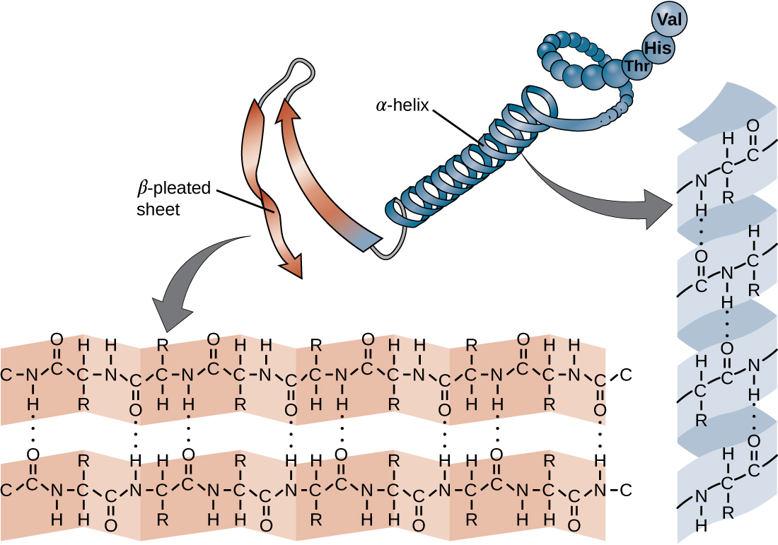
Fig. 1.13 α-helices and β-sheets are stablized by hydrogen bonds (the dotted lines) between the backbone of proteins, i.e., the side chains are not involved. The hydrogen bonds form between the oxygen atom in the C group in one amino acid and the hydrogen in the N group. Credits: CC BY 4.0 modified from [OpenStax College, n.d.].

Turns are short secondary structure elements that are stabilized by hydrogen bonds between amino acids that are 1 to 5 peptide bonds away. The most common form are β-turns, which connect antiparallel β-strands.

Note 1.2: Secondary structure amino acid preference

Although secondary structure elements are formed by hydrogen bonds between the backbone, certain amino acids are favoured in secondary structures and others are disfavoured. For example, methionine, alanine, leucine, and glutamic acid are favoured in α-helices, whereas proline, glycine, and tyrosine are disfavoured. Also, valine, isoleucine, tyrosine, cysteine, tryptophan, phenylalanine, and threonine are more frequently found in β-sheets, compared to α-helices. In turns, glycine, asparagine, proline, and serine are preferred. These preferences are used to predict secondary structure elements in proteins (see chapter 4).

The peptide bond is very rigid and planar, i.e., it cannot rotate to form the elements of protein structure. However, the N-C_α and the C_α-C bonds can freely rotate, being only limited by the size and properties of the R-groups. The 3D shape of the polypeptide backbone is thus determined by two torsion angles: phi (φ) between N and C_α and psi (ψ) between C_α and C (Fig. 1.14A). Although φ and ψ can rotate in principle, steric hindrance prevents certain combinations of angles, i.e., the bulkiness of the R-groups restricts the possible conformations. Thus, certain combinations of φ and ψ are preferred. We can plot the combinations of φ and ψ in a protein, in a so-called Ramachandran plot (Fig. 1.14B).

The regular secondary structure elements (α-helix and β-sheet) contain consecutive amino acids with similar (φ,ψ) values. These regions are typically highly populated in a Ramachandran plot. Thus, the Ramachandran plot can be used to assess how plausible a predicted protein structure is.

Fig. 1.14 A) The φ, and ψ torsion angles of a polypeptide chain. Credits: CC BY-NC 4.0 [Ridder et al., 2024]. B) A typical Ramachandran plot. The red regions marked do not have any steric hindrance, yellow areas represent conformations that have steric hindrance, light yellow areas represent conformations that are generally sterically unfavorable, and white areas do not have any allowed conformations. Credits: Ramachandran plot modified from PROCHECK [Laskowski et al., 1993].

See also

An illustrative animation on φ and ψ.

---

Tertiary structure

The tertiary structure of a protein describes the complete folding of an entire polypeptide chain. In contrast to the secondary structure, the tertiary structure of a protein involves interactions between the amino acid’s side chains that can occur at short-range and long-range (Fig. 1.15). Thus, the chemical properties of the amino acids are very important for the tertiary structure. Different types of interactions stabilize the tertiary structure:

• Hydrogen bonds involving polar amino acids.

• Ionic bonds between positively and negatively charged amino acids.

• Hydrophobic R groups that tend to lie in the protein’s interior, stabilized by hydrophobic interactions.

• Disulfide bonds (i.e., covalent bonds between cysteines).

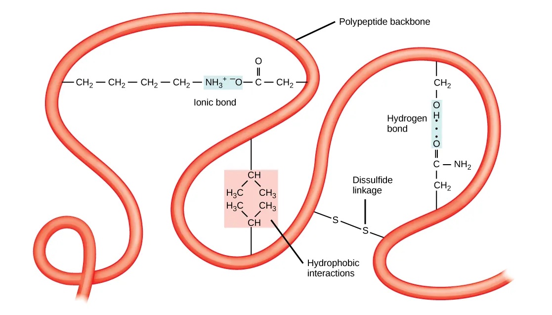
Fig. 1.15 Chemical interactions that stabilize the tertiary structure of proteins. Credits: CC BY 4.0 [Clark et al., 2018].

Note 1.3: Denaturation

The noncovalent bonds that stabilize the protein structure are broken at high temperature. Thus, most proteins unfold above about 60°C. This process is called denaturation and is generally irreversible. When proteins denature, they lose their function.

Domains are distinct functional and/or structural units in a protein and are typically 50 to 350 amino acids long. Usually, a domain is responsible for a particular function or interaction, contributing to the overall role of a protein. A domain can exist in different contexts with other domains (Fig. 1.16). In a multidomain protein, each domain folds independently of the others.

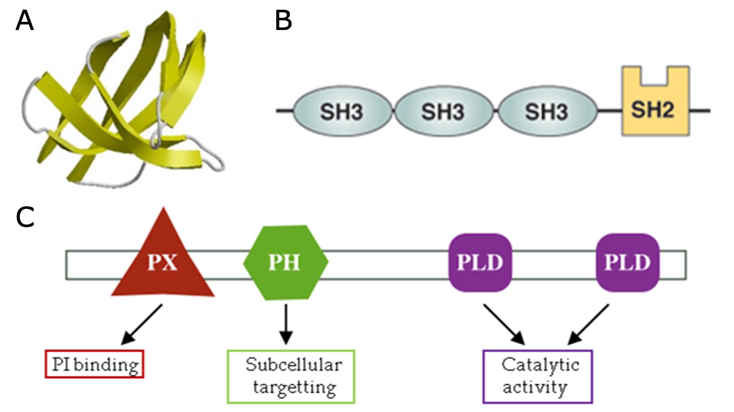
Fig. 1.16 A) Example of an Src homology 3 (SH3) domain that is involved in protein-protein interaction. SH3 domains occur in a diverse range of proteins with different functions. B) The cytoplasmic protein Nck contains multiple SH3 domains. C) Domain composition of phospholipase D1, which has multiple functional domains that contribute to its overall function. Credits: CC BY 4.0 [Sangrador, 2023].

---

Quaternary structure

Finally, individual folded polypeptides can interact to form protein complexes, also called quaternary structures. The quaternary structure is stabilized by the same types of interactions as the tertiary structure. The difference is that the amino acids involved belong to different polypeptides.

Many functional proteins are composed of multiple subunits, they are also called oligomers (Fig. 1.17). The subunits can originate from the same protein sequence (called a homomer) or from different sequences (called a heteromer). Proteins consisting of two subunits are also called dimer.

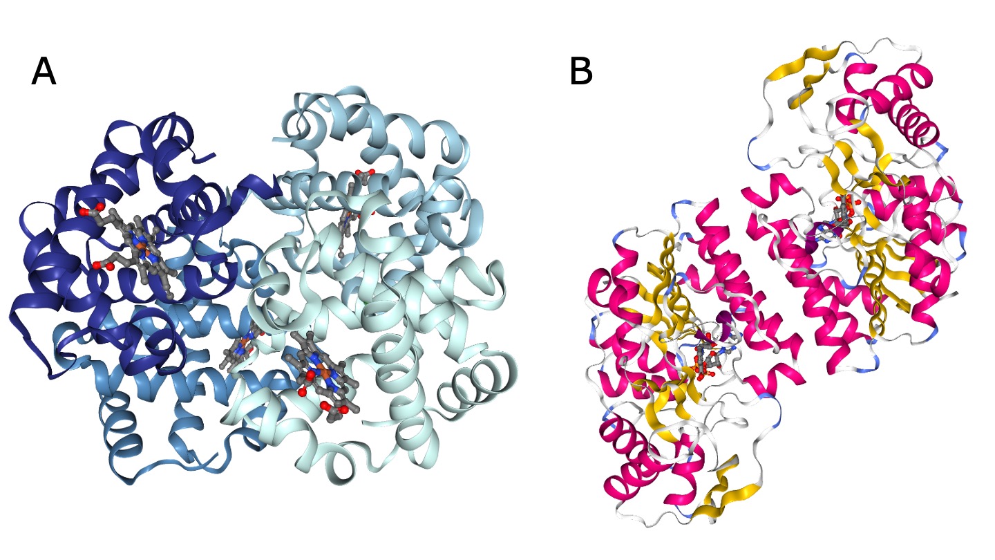
Fig. 1.17 Examples of oligomers. A) Myoglobin, a heteromer of four subunits (PDB structure 1HV4 colored by chain). Credits: [Berman et al., 2000, Liang et al., 2001, Rose et al., 2018]. B) UDP-galactose 4-epimerase, a homodimer (PDB structure 1EK5 colored by secondary structure). Credits: [Berman et al., 2000, Rose et al., 2018, Thoden et al., 2000].

---

Substitutions

Mutations in the gene sequence can lead to changes in the primary structure of the protein, e.g., a substitution of one amino acid by a different one. Often, such substitutions still lead to highly similar protein structures that perform a similar or even the same function, especially when the exchanged amino acids have similar chemical properties. Nevertheless, single amino acid substitutions can have severe consequences. A prominent example is sickle cell anemia, where a substitution of valine to glutamic acid in hemoglobin β results in a structural change that leads to a distortion in red blood cells (Fig. 1.18).

Fig. 1.18 Consequences of a substitution in hemoglobin β resulting in sickle cell anemia. Credits: Rao, A., Tag, A. Ryan, K. and Fletcher, S. Department of Biology, Texas A&M University.

---

Visualization

There are many styles to view protein molecular structures. Some styles focus on detailed chemical structure, others are targeted at the protein surface. For some examples see Fig. 1.19.

Fig. 1.19 Different representations of the PDB structure 5PEP generated with NGL. Credits: [Berman et al., 2000, Rose et al., 2018, Cooper et al., 1990].

See also

Most of the figures in this section are taken from OpenStax, where you can also find more information on proteins.

---

Genome annotation

Genome annotation is the process of deciphering what information is encoded in an organism’s DNA. It is an ongoing effort in organisms with known genome sequences. Even moreso, genome annotation is a critical step in acquiring biological insights from newly sequenced genomes. Given the large size of any genome, automated procedures are used to identify various genomic elements such as genes, regulatory regions, transposable elements, or other non-coding elements. Each of these bioinformatic procedures typically focuses on identifying one type of element, and as such a complete genome annotation project can be thought of as a pipeline of various procedures. The following section describes the most common steps in genome annotation.

Note 1.4: Alignment algorithms

Several steps in the genome annotation process make use of algorithms that can search or align biological sequences, for example the BLAST algorithm. Chapter 2 covers sequence alignment and search in greater detail. For now, it is sufficient to know that these algorithms can quickly search very large collections of biological sequences to identify sequences that look similar (what we mean exactly by ‘similar’ is also part of chapter 2).

Repeat masking

Repeat masking involves the identification and masking (hiding) of repetitive sequences within a genome. It is an essential first step in annotating most genomes because repetitive sequences can pose significant challenges in genome annotation. Masking repeats generally improves:

• Accuracy: repetitive elements can be mistakenly annotated as genes or other functional elements, leading to inaccurate predictions and interpretations of the genome.

• Computational efficiency: identifying and processing repetitive sequences can be computationally intensive. However, masking these repetitive regions reduces the computation time of all downstream analyses.

• Biological relevance: repetitive sequences are usually not involved in the coding of proteins of interest. Therefore, focusing on non-repetitive regions is a smart choice in understanding the genes and regulatory elements that drive biological processes.

Most repeat masking workflows work by first compiling (or using a precompiled) ‘repeat library’: a collection of known repetitive elements that have previously been characterized. Subsequently, the genome to be annotated is compared against this repeat library using various computational algorithms, such as BLAST or RepeatMasker. When a match is found, the corresponding region in the genome is ‘masked’ or annotated as a repetitive element. This means that these regions are excluded from further analysis or labeled as repetitive.

Gene prediction

The process of finding protein coding genes differs between prokaryotic and eukaryotic genomes. In both cases the aim is to find open reading frames (ORFs): contiguous stretches of DNA that encode proteins. However, since RNA splicing (Fig. 1.6) is almost absent in prokaryotic genomes, prokaryotic ORFs can be found directly in the genomic DNA. As a result, simply enumerating all possible ORFs in a genome is a common step in prokaryotic genome annotation. In contrast, ORFs in eukaryotic genomes are found on mature mRNAs. As such, all eukaryotic gene prediction methods take splicing into account, thereby greatly increasing their computational complexity. Both prokaryotic and eukaryotic gene prediction typically can be classified as either evidence based prediction or ab initio prediction, both will be explained below.

Evidence based prediction

This data-driven approach uses existing and newly generated data to get hints on what regions of a genome encode genes. Depending on the type of data, these predictions have more or less predictive power. Some commonly used evidence types are:

• RNA-sequencing data: the most direct form of evidence for what regions of the genome are transcribed. As such, RNA-sequencing (often abbreviated to RNA-seq) ‘reads’ often provide the best form of evidence in identifying splice sites in eukaryotes. Note that not all transcribed RNA will be translated into proteins, and that therefore not all RNA-sequencing reads are evidence for protein coding genes. Distinguishing between protein-coding and non-coding RNA is not always trivial.

• Homology evidence: Aligning DNA or protein sequences of known genes (from other organisms) is valuable evidence in finding coding regions of the genome. Due to the redundancy in the genetic code, it is not trivial to correctly identify splice sites when aligning protein sequences to a genome. Homology evidence from closely related organisms leads to higher quality predictions than evidence from distantly related organisms.

• Whole-genome alignments: this approach uses the annotated genome of a closely related organism to directly identify coding regions in a novel genome. For example: whole-genome alignment of mouse and human genomes reveals that large parts of mouse chromosome 2 are homologous to human chromosome 20. The alignment procedure results in a direct 1-to-1 mapping of mouse and human genome coordinates, and as such annotation coordinates can be transferred between genomes.

Ab initio prediction

Ab initio (latin): from first principles, from the beginning

These methods rely on statistics to learn a predictive model from a known annotated genome. Various forms of ab initio models exist, and whereas implementation details differ, most follow a similar line of reasoning. For now, we will stick to a high level description. All ab initio models scan through a DNA sequence and at each position give a score for a specific type of annotation. In addition, they often take their genomic context into account. For example, the probability of a protein-coding annotation on a nucleotide A is high when the next two observed nucleotides are T and G, producing the ATG start-codon methionine. In addition, most methods also take the predicted annotation of the genomic context into account. For example: the probibility that ATG actually codes for a start codon is much higher if we can predict an in-frame stop codon. In eukaryotic genome prediction these models become quite complex because they have to include splice sites in all three reading frames. How exactly a model decides what annotation score to give to which nucleotide is part of the model architecture and parameterization. In all cases, the model parameters are chosen to accurately reproduce a known genome annotation. If sufficient data is used to learn the model parameters, it is assumed that these models can be used to predict annotations on novel genome sequences. Like homology-based prediction, this model-based approach works best for closely related organisms. In the past, almost all ab initio prediction methods were formulated as hidden Markov models (HMMs) (see Note 1.5). Examples of tools implementing HMM based ab initio prediction are SNAP, GeneMark, and Augustus. With the availability of more high quality data (genome sequences and accompanying annotations), approaches based on deep learning and generative AI have proven to frequently perform better than HMM based approaches.

Note 1.5: Hidden Markov models (HMMs)

Hidden Markov models (HMMs) are useful for the statistical modelling of general sequence characteristics. As such they find widespread adoption in bioinformatics to study biological sequences. Providing a full technical description of all aspects of HMMs is outside of the scope of this book. Here we will stick to a somewhat simplistic description to provide a first introduction.

A hidden Markov model can be used to predict some unobserved labelling across a sequence of observations. For example: in genome annotation, coding and non-coding regions of a genome can be treated as an unobserved characteristic, where the nucleotides are the sequence of observations. As such, ‘hidden’ refers to the unobserved labelling. In addition, ‘Markov’ refers to some useful statistical assumptions on the nature of independence between observations and labellings that enable efficient computation.

More formally, the unobserved labellings are referred to as the ‘hidden states’, and every hidden state contains some probabilities of observing our sequence of interest, called the ‘emission probabilities’. To complete our HMM definition, we define ‘transition probabilities’ between hidden states.

The combination of hidden states, emission probabilities, and transition probabilities enable asking questions such as ‘given my current observation and a certain label of my previous observation, what is the most likely label for my current observation?’. In the context of genome annotation this would translate to for example ‘given that I see a stop-codon, and that my previous label was coding sequence, what is my current most likely label?’, the answer to which would be ‘non-coding’ (See Fig. 1.20).

Fig. 1.20 A: Graphical representation of a general hidden Markov model. Shaded circles indicate observations, white circles indicate unobserved labellings (hidden states). Black arrows indicate transition probabilities between hidden states, and emission probabilies for observations from hidden states. Note that there are no arrows between observations! This is one of the properties of HMMs that enable efficient computation. B: A (simplified) HMM variant that labels a sequence of DNA codons as either coding or non-coding. Real-world gene predicition HMMs use a more elaborate structure with more hidden states, and six-frame representations of the DNA. Credits: CC BY-NC 4.0 [Ridder et al., 2024].

Chapter 2 and Chapter 4 cover various other applications of HMMs in bioinformatics, such as defining and prediction sequence domains, or transmembrane properties of proteins.

Evidence/prediction integration

From the previous sections it has now become clear there are several ways of predicting what the genes in a genome look like. Since these various approaches almost never agree exactly in their predictions, a final step in genome annotation is evidence and prediction integration. Typically a weighted consensus approach is used: each individual source of evidence is given a weight representing how much it should influence the final decision, after which a majority vote decides what the annotation should look like. Typically RNA-seq evidence gets a high weight, and various forms of homology evidence can be weighted depending on how closely related they are to the genome of interest.

Functional annotation

So far, all described steps in the genome annotation process have dealt with what genes look like on a structural level. To gain biological insight, the next step is to assign functional annotations to the predicted genes. This functional annotation step consists of using various sequence alignment and search tools to find sequences with a known function/description and to transfer the information of the known gene to the predicted gene. Several databases of high-quality known functions are often used, which are described in more detail in the next section of this chapter. In Chapter 2 we will learn about approaches how to search these databases efficiently.

Note 1.6: Visualizing gene structure

Gene models: the genomic structure of a gene (often referred to as a gene ‘model’) is typically visualized by a set of lines and rectangles with predefined meaning.

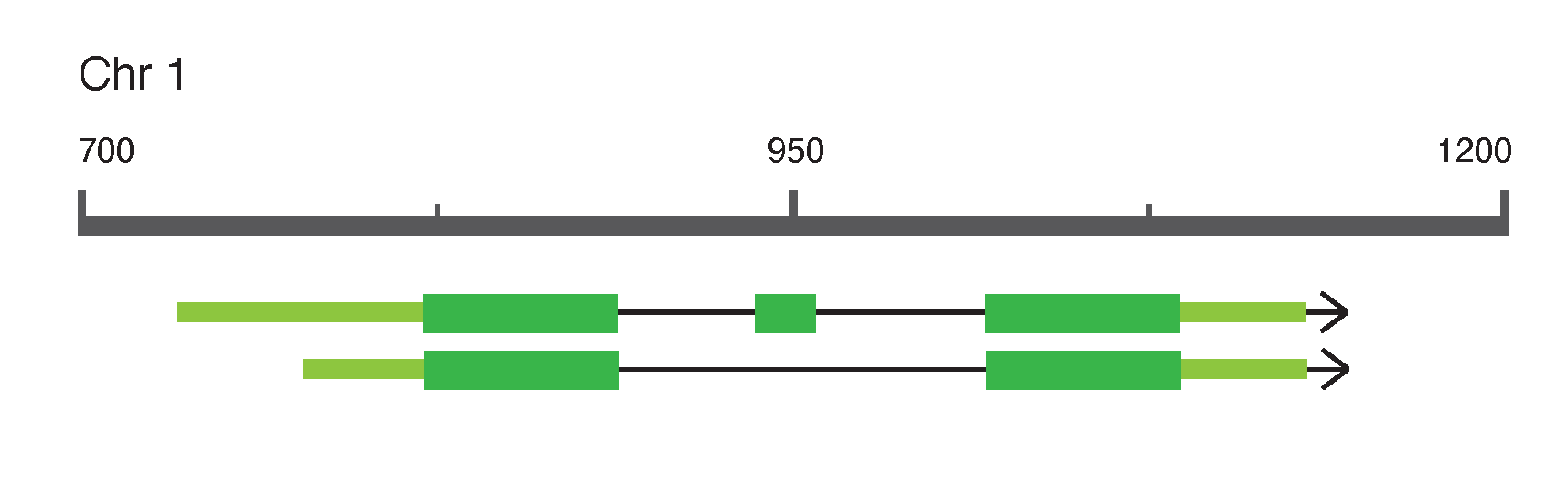
Fig. 1.21 An example gene model. Various visualization conventions can be identified: boxes represent genomic regions that are transcribed. Boxes are exons, lines between boxes are introns. Narrow boxes (sometimes with a lighter color) are untranscribed regions (UTRs), wider boxes (sometimes darker colored) are coding sequence regions (CDS). The arrow indicates the direction of transcription. In this example a gene on chromosome 1 with two splice variants is shown, where the first variant has a slightly longer 5’ UTR and an additional CDS exon in between the first and last exons. Credits: CC BY-NC 4.0 [Ridder et al., 2024].

Genome browsers facilitate interactive visualization of annotations and evidence alignments on genome sequences. Various implementations exist, but all genome browsers typically provide a linear view of a chromosome that can be scrolled and zoomed. In addition, various annotation ‘tracks’ can often be toggled, to display for instance known gene structures, RNA sequencing alignments, or homologous protein sequence alignments. Most visualization elements can be clicked to open pop-up windows with additional information.

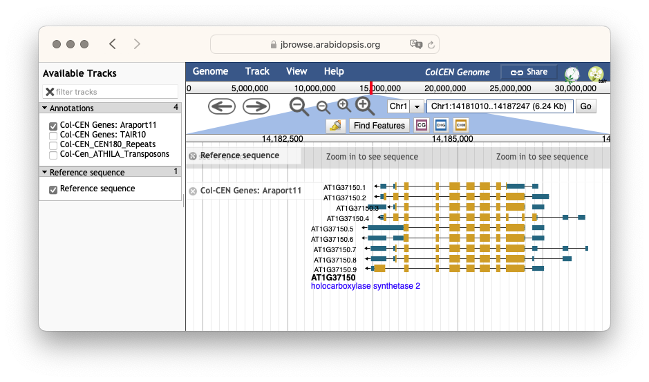
Fig. 1.22 A screenshot of the JBrowse genome browser showing Arabidopsis thaliana chromosome 1 with a gene that has multiple splice variants. Credits: [Buels et al., 2016].

---

Databases

Introduction

Databases are at the core of bioinformatics. In all analyses, we integrate pre-existing data and we need to access this data. The journal Nucleic Acids Research publishes an entire issue in the beginning of each year on new and updated databases. The list of these databases can also be accessed online.

Computer scientists have developed different kinds of databases. One example are relational databases, which can be queried by SQL (structured query language) and which perform well for data that is processed computationally. Another example are XML (extended markup language) databases which store data in specified well-structured XML files. Nevertheless, most databases for biological sequence data use flat file databases, where the data is saved in structured text files. This data can be manipulated in a text editor without requiring an additional program for database management, and they can be easily exchanged between scientists. On the downside, searching them has a lower performance. This is why they are often indexed, i.e., they contain an index of keywords, similar to a glossary in a book.

Depending on the kind of data included, we distinguish different kinds of biological databases:

• Primary databases contain primary sequence information from experimentally derived data that is directly submitted by the scientists that generated the data.

• Secondary databases provide the results of analyses of the information in primary databases.

Each entry in a database has a unique accession number. This number is permanent and provides an unambiguous way to link to the entry. The information that the accession refers to should not change. To still allow updates to an entry, the accession number can contain a version, usually after a dot. For example, NC_003070.9 is the latest version (version 9) for Arabidopsis thaliana chromosome 1 in RefSeq.

Database entries often link to each other via cross links.

See also

Ten Simple Rules for Developing Public Biological Databases contains additional reading material on what it takes to properly maintain a public database service.

---

GenBank

GenBank is a popular primary database for nucleotide sequences and is based at the NCBI (National Center for Biotechnology Information). A GenBank release usually occurs every two months and the most recent release from the 15^th of December 2023 contains ~250 million sequences and additionally ~3.7 billion WGS (whole genome shotgun) records. The latter are genome assemblies or genomes that were not yet completed. The complete database is available for download via FTP, but the most convenient way to access individual entries is via the search on the GenBank website (Fig. 1.23).

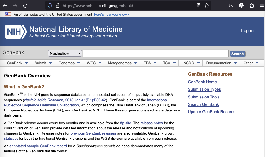
Fig. 1.23 A screenshot of the GenBank website. Credits: [Benson et al., 2012].

Additional information

These days, it is required for publication in most peer-reviewed journals that scientists submit their sequence data to GenBank or an associated database, alongside sufficiently informative meta-data that describes how the data was generated.

Since data is directly submitted to GenBank, the information for some loci can be highly redundant. The sequence records are owned by the original submitter and cannot be altered by someone else.

Note 1.7: Database redundancy

‘Redundancy’ in the context of a database refers to identical data that is present more than once. Typically, metadata is not taken into account when determining redundancy. Example: two different labs have determined the DNA sequence of a bacterial gene involved in some disease. The metadata will be different, but the sequence data will be identical, so these two database records are redundant.

NCBI hosts several databases that are classified as ‘non-redundant’, for example RefSeq non-redundant proteins. Here, redundancy is defined so that a ‘non-redundant protein record always represents one exact sequence that has been observed once or many times in different strains or species’.

Genbank is part of the INSDC (International Nucleotide Sequence Database Collaboration). The other two member databases are ENA (European Nucleotide Archive) and DDBJ (DNA Data Bank of Japan). The data submitted to either database is exchanged daily, so all databases contain essentially the same information.

---

RefSeq

The Reference Sequence (RefSeq) collection is also hosted at NCBI and contains genomic DNA, transcripts, and proteins. The aim of RefSeq is to provide non-redundant, curated data. RefSeq genomes are copies of selected assembled genomes in GenBank. Additionally, transcript and protein records are generated by several processes:

• Computation via the eukaryotic or prokaryotic annotation pipeline.

• Manual curation.

• Transfer of information from annotated genomes in GenBank.

  In contrast to GenBank, RefSeq records are owned by NCBI and can be updated to maintain annotation. The current release is 222 from the 8^th of January 2024 and contains ~305 million proteins from ~145,000 organisms.

The RefSeq accessions directly provide information on molecule types. For example, NC_ accessions denote complete genomes, NP_ accessions denote proteins in one genome, and WP_ accessions denote proteins in multiple genomes.

---

UniProt

There is lots of information available for proteins, such as sequence information, domains, expression, or 3D structure. The aim of the Universal Protein Resource (UniProt) is to provide a comprehensive resource for proteins and their annotation. UniProt contains three databases (Fig. 1.24):

• UniProt Knowledgebase (UniProtKB) - see below.

• UniProt Reference Clusters (UniRef - clusters of protein sequences at 100%, 90%, and 50% identity.

• UniProt Archive (UniParc - non-redundant archive of publicly available protein sequences seen across different databases.

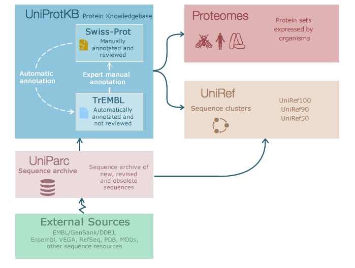
Fig. 1.24 The information flow in Uniprot. Credits: CC BY-NC-ND 4.0 [Leon and Pastor, 2021].

UniProtKB is the central hub for functional information on proteins. For each protein it contains the core data (such as sequence, name, description, taxonomy, citation) and as much annotation information as possible. It contains many cross-references to other databases and is generally a very good starting point to find information on a protein.

UniProtKB consists of two sections:

• Swiss-Prot - manually-annotated records with information extracted from literature and curated computational analysis.

• TrEMBL - automatically annotated records that are not reviewed.

UniProtKB is updated every 8 weeks. The current release has ~570,000 entries in Swiss-Prot and ~248 million entries in TrEMBL.

---

Prosite

Prosite is a secondary database of protein domains, families, and functional sites. Some regions in protein families are more conserved than others because they are important for the structure or function of the protein. Prosite contains motifs and profiles specific for many protein families or domains. Searching motifs in new proteins can provide a first hint for protein function.

The current release of Prosite from the 24^th of January 2024 contains 1311 patterns, 1386 profiles, and 1400 ProRule entries.

A Prosite pattern is typically 10 to 20 amino acids in length. These short patterns are usually located in short well-conserved regions, such as catalytic sites in enzymes or binding sites. A pattern is represented as a regular expression, where amino acids are separated by hyphens and x denotes any letter. Repetitions can also be given as the number of repetitions in brackets. For example, [AC]-x-V-x(4)-{ED} matches sequences that contain the following amino acid sequence: Ala or Cys-any-Val-any-any-any-any-any but Glu or Asp. Note that this representation is qualitative, a sequence either matches a pattern or it does not.

Patterns cannot deal with mismatches and are limited to exact matches to the pattern. Thus, they are not well suited to identify distant homologs. A Prosite profile is more general than a pattern and can also detect poorly conserved domains or families. They characterize protein domains over their entire length and do not just model the conserved parts. Profiles are estimated from multiple sequence alignments and we learn more about them in chapter 2. For now, it is important to know that profiles model matches, insertions, and deletions. Importantly, profiles are quantitative representations, they will return a score how well the sequence fits to the profile. A threshold can be applied to get high-scoring profiles for a sequence. In contrast to patterns, a mismatch to a profile can be accepted if the rest of the sequence is highly similar to the profile. Profiles are well suited to model structure properties of a domain.

Notably, profiles cover the structural relationships of domains, but they might also score a sequence highly that lacks important functional residues. To include that information, ProRule contains additional information about Prosite profiles, such as the position of structurally or functionally important amino acids. ProRule is used to guide curated annotation of UniProtKB/Swiss-Prot.

InterPro

The Integrated Resource of Protein Families, Domains and Sites (InterPro) integrates 13 member databases (including Prosite and Pfam) into a comprehensive secondary database. Additionally, it provides annotation from other tools, for example to annotate signal peptides and transmembrane regions. It allows to identify functionally important domains and conserved sites in a sequence by simultaneously annotating it using the member databases. Interpro can be used to find out which protein family a sequence belongs to, or what its putative function is. Additionally, one InterPro entry can integrate entries from the member databases, if they represent the same biological entity, reducing redundancy. InterPro entries are also linked to Gene Ontology. They are curated before being released.

InterPro is updated every 8 weeks. The current release from the 25^th of January 2024 contains ~41,000 entries, which represent different types:

As an example, look at the InterPro entry for the type 2 malate dehydrogenase protein family. The entry has a name (malate dehydrogenase, type 2) and accession (IPR010945). The contributing entries in member databases are shown on the right-hand side, with links to the individual member database entries. A descriptive abstract explains what these proteins are and what their function is. A set of GO terms is also provided, which describe the characteristics of the proteins matched by the entry.

You can get the InterPro annotation for a protein by running a new sequence search (Fig. 1.25), or by by looking up its UniProt accession (Fig. 1.26).

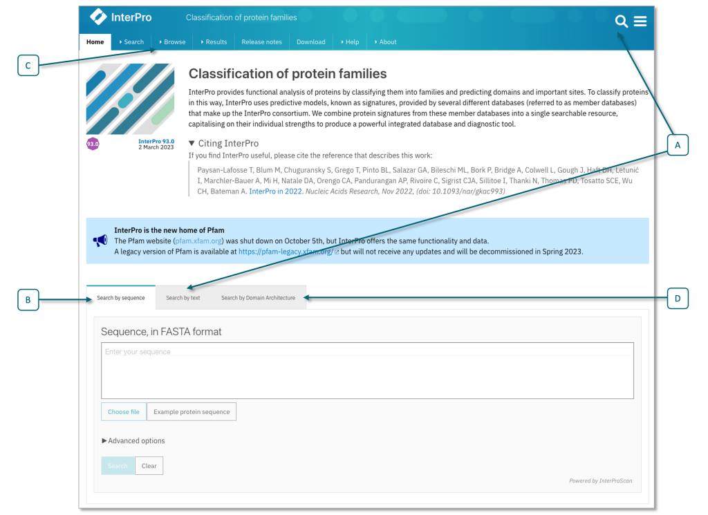
Fig. 1.25 Search fields on the InterPro home page, showing text search field (A) and the sequence search (B) options, including ‘Advanced options’, where you can limit your search to member databases or sequence features of interest. Selecting the browse tab in the top menu © allows access to a browse search, (e.g., search for member database signature, InterPro entry type), see also Fig. 1.26. You can also search for a particular domain architecture (D). Credits: [Paysan-Lafosse et al., 2022].

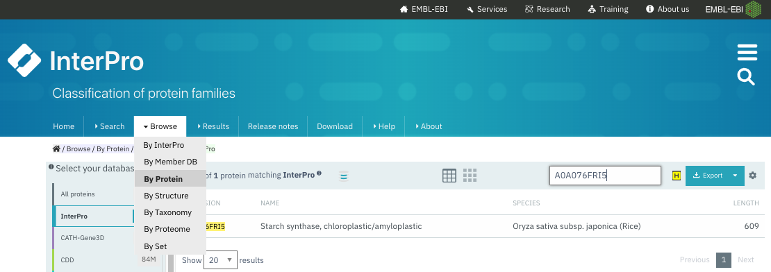
Fig. 1.26 Browse the annotated proteins in Interpro and search for a UniProt accession. See resulting entry in (Fig. 1.27). Credits: [Paysan-Lafosse et al., 2022].

Fig. 1.27 The result page when looking up UniProt accession A0A076FRI5 in InterPro. You can see the family and domain annotation and on the right the accessions in InterPro and in the member databases. You can click on each of these accessions to get to the entry information. Credits: [Paysan-Lafosse et al., 2022].

You may have noticed a colored letter before each InterPro accession, e.g., F before IPR011835 or D before IPR001296 (Fig. 1.27). These icons denote the different InterPro entry types:

• (Homologous) Superfamily - a large diverse family, usually with shared protein structure.

• Family - a group of proteins sharing a common evolutionary origin, reflected by their related functions and similarities in sequence or structure.

• Domain - a distinct functional or structural unit in a protein, usually responsible for a particular function or interaction.

• Repeat - typically a short amino acid sequence that is repeated within a protein.

• Site - a group of amino acids with certain characteristics that may be important for protein function, e.g., active sites or binding sites

Fig. 1.28 The icons for the different InterPro entries (homologous superfamily, family, domain, repeat or site). Credits: CC BY-SA 4.0 [Mitchell, 2020].

See also

You can find more information on InterPro entry types with examples here.

Pfam

Pfam is an important resource for protein domains. In Pfam, domains are classified according to profiles that are modelled as Hidden Markov models (HMMs). We will learn more on HMMs in chapter 2.

Pfam is now integrated in InterPro. Each Pfam domain can be represented with a logo, where the amino acids frequent at a particular position are represented as larger letters (Fig. 1.29).

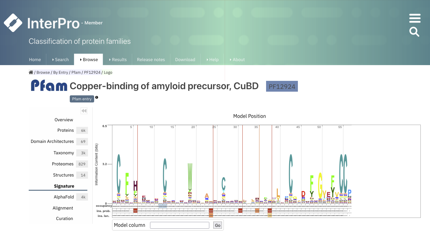
Fig. 1.29 The Pfam logo for PF12924. Credits: [Paysan-Lafosse et al., 2022].

---

File formats

There are many different formats for biological data. A format is a set of rules about the contents and organization of the data. You should be familiar with a couple of common data formats in bioinformatics, which you will experience in the practicals.

Note 1.8: Examples of common data formats in bioinformatics

• FASTA

• Genbank

• GFF (Generic Feature Format)

• FASTQ

• SAM/BAM (Sequence Alignment/Map format)

• VCF (Variant Call Format)

• PDB (structure data)

Plain text files

Many of the biological data formats are plain text files, they only contain letters, numbers, and symbols, but no formatting, such as font size or colors. As a convention, they usually have the ending .txt. The advantage of plain text files is that they can be opened with any text editor on any computer. Plain text differs from rich text format, where the latter can also include formatting. Many bioinformatics programs expect plain text files as input. Thus, when creating them on your computer, take care to save in this format, and not for example in rtf or word.

On a Windows computer, plain text files can for example be created with the Notepad program (Fig. 1.30).

Fig. 1.30 A screenshot of Notepad on Windows. Credits: CC BY-NC 4.0 [Ridder et al., 2024].

On a Mac, plain text files can for example be created with the TextEdit program (Fig. 1.31). Take care to set the settings to plain text.

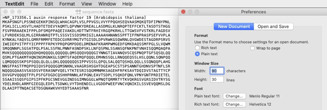
Fig. 1.31 A screenshot of TextEdit on Mac. Credits: CC BY-NC 4.0 [Ridder et al., 2024].

See also

If you are not yet familiar with plain text editors, then try it now and write and save a plain text file on your computer!

There are some important file formats in bioinformatics. A fasta file stores a DNA or protein sequence (Fig. 1.32). Information on the sequence is found in the header (starting with >), which is on one line and the sequence can go over multiple lines. A multi-fasta file stores multiple sequences.

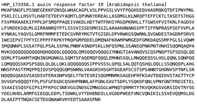
Fig. 1.32 A sequence in fasta format. Credits: CC BY-NC 4.0 [Ridder et al., 2024].

The GenBank file format is a popular format to represent genes or genomes. Here you can find an example GenBank record with annotations. Important elements are the Locus, Definition (i.e., the name), and the Organism. Additionally, Features, such as genes and CDSs (coding sequences) are listed.

Binary files

Binary files are all the files that are not text files, they cannot be opened in a text editor. Instead, they need special programs to write and to open and interpret them. Examples are word files (.docx) which can be opened with Word, pdf files (.pdf) which can be opened with Acrobat Reader, or image files (e.g., .png) which can be opened with image viewers.

Binary files are are also sometimes used in bioinformatics. Examples include the bam format, which is a binary version of the sam format or the gzip format. Gzip is used for compressing text files without the loss of information. For large files, lots of disk space can be saved this way.

---

Ontologies

An ontology is a comprehensive and structured vocabulary for a particular domain, such as biology, genetics, or medicine. It defines the various terms used in a domain, along with their meanings and interconnections. As such, ontologies serve as standardized frameworks for organizing and categorizing information in a way that enables effective communication and reasoning among researchers, practitioners, and computer systems. For example, the terms in an ontology can encompass biological entities like genes, proteins, and cells, as well as processes, functions, and interactions that occur within living organisms. Most of the databases mentioned mentioned in this chapter use ontologies in some way to describe their data.

Ontologies play a crucial role in bioinformatics because they facilitate:

1. Standardization and consistency: ontologies provide a common language and consistent framework for researchers and professionals, ensuring that everyone understands and uses terms in the same way.

2. Interoperability: ontologies facilitate the sharing and integration of data and knowledge across different research groups, institutions, and databases. They enable computer systems to process data more accurately, leading to more meaningful analyses and discoveries.

3. Scientific reasoning: by organizing information in a logical and structured way, ontologies help researchers generate hypotheses, design experiments, and validate findings more effectively.

Note 1.9: FAIR principles

As described above, ontologies facilitate scientific reproducibility. A key concept in scientific reproducibility are the FAIR principles, with FAIR standing for Findable, Accessible, Interoperable, and Reusable. This reader does not describe them in detail, but you should read the following online resource to familiarize yourself with the FAIR principles.

Ontologies typically form a hierarchy, where specific terms point to more generic terms. More generally, most ontologies are represented as a graph, where ontology terms are the nodes and relationships between terms are edges. As such, one ontology term may have more than one parent term.

A variety of ontologies are frequently used in the life sciences, some of which are discussed in greater detail below.

Gene Ontology

The Gene Ontology (GO) is a knowledgebase for the function of genes and gene products (e.g. proteins). It is organised into three different domains covering various aspects:

• Molecular Function: molecular-level functions performed by gene products (e.g. proteins), such as ‘catalysis’ or ‘transport’. Most molecular functions can be performed by individual gene products, but some functions are performed by complexes consisting of multiple (possibly differing) gene products. GO molecular functions often include the word “activity” (an amylase enzyme would have the GO molecular function amylase activity).

• Cellular Component: the cellular structures (or location relative to them) in which a gene product performs its function. Can be cellular compartments (e.g., mitochondrion) or macromolecular complexes of which they are part (e.g., the ribosome).

• Biological Process: the larger biological programs composed of multiple molecular activities, for example DNA repair or signal transduction.

Note 1.10: Molecular pathway?

A biological process is not equivalent to a molecular pathway. At present, the gene ontology does not represent the dynamics or dependencies that would be required to fully describe a pathway.

A good example of how ontologies are represented as graphs is the biological process hexose biosynthetic process, which has two parents: hexose metabolic process and monosaccharide biosynthetic process. This reflects that biosynthetic process is a subtype of metabolic process and a hexose is a subtype of monosaccharide. (Fig. 1.33).

Edges between GO terms in the GO hierarchy can represent various relationships between genes and gene products. The four main relationship types used in the gene ontology are ‘is a’, ‘part of’, ‘has part’, and ‘regulates’ (see Fig. 1.34).

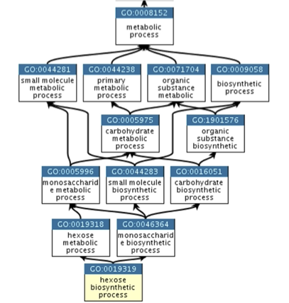
Fig. 1.33 An extract of the Gene Ontology hierarchy. Credits: [Binns et al., 2009]

Sequence Ontology

The Sequence Ontology (SO) describes biological sequence elements such as genes or repeats, along with their features and attributes.

The sequence ontology is organized on four main levels:

• Attribute: an attribute describes a certain quality of a given sequence, for example the sequence source (i.e., how it was generated).

• Collection: multiple discontiguous sequences together, for example the chromosomes of a complete genome.

• Feature: the most general top-level entry that describes any extent of a continuous biological sequence, for example a gene is a region, which in turn is a sequence feature.

• Variant: intended to describe genetic variation. The definition of a sequence variant is composed of other entries in the sequence ontology: “A sequence_variant is a non-exact copy of a sequence_feature or genome exhibiting one or more sequence_alterations”

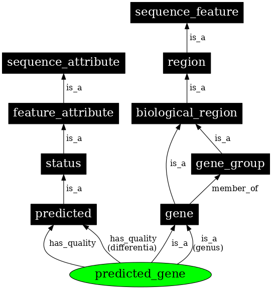
Fig. 1.34 An extract of the Sequence Ontology hierarchy. Credits: [Eilbeck et al., 2005].

Other ontologies

Many more ontologies exist and are relevant to biomedical research. The European Bioinformatics Institure (EBI) provides an ontology lookup service that facilitates searching for ontologies. Examples of other ontologies are the plant ontology that describes various anatomical structures in plants, and the human disease ontology.

---

Practical assignments

This practical contains questions and exercises to help you process the study materials of Chapter 1. You have 2 mornings to work your way through the exercises. In a single session you should aim to get about halfway through this guide (i.e., day 1: assignment 1-3, day 2: assignment 4 and project preparation exercise). Use the time indication to make sure that you do not get stuck in one assignment. These practical exercises offer you the best preparation for the project. Especially the project preparation exercise at the end is a good reflection of the level that is required to write a good project report. Make sure that you develop your practical skills now, in order to apply them during the project.

Note, the answers will be made available after the practical!

\pagebreak

Assignment I: DNA/Genes (45 minutes)

1. How do you distinguish a ribose sugar from a deoxyribose?

2. Which bases are purines?

3. What is the complementary base of A? C? G? T?

4. What is the reverse complement of sequence ACGGTGATC?

5. What is the GC content of sequence ATCGATCGGC?

6. Which is correct? A nucleotide sequence is written from:
   A. 5’ to 3’
   B. 3’ to 5’

7. In a DNA sequence the G stands for:
   A. Glycine
   B. Guanine
   C. Glucose
   D. Glutamic acid

8. Given a coding DNA strand. Write down the non-coding strand, the transcribed sequence, and the resulting chain of amino acids. You may use Fig. 1.3.

Coding strand:         5' ATGGTTTTACTTGAA 3'
Non-coding strand:     ......................
mRNA:                  ......................
Amino acids:           ......................

9. On your computer, browse to UniProt and search for UniProt ID B3H4Y2.
   a. In which organism is this protein found? What is the length of this protein? What is the corresponding gene ID?
   b. Write down the first 5 and last 5 amino acids of the protein.

10. Browse to arabidopsis.org and click on “JBrowse” (Firefox or Chrome recommended). This will take you to a genome browser of the Arabidopsis genome. Search for the gene ID from question 9 (see screenshot above). Under “Help” -> “General” you can find some information to help you understand what you are looking at.
    a. You can see that this gene produces two different mRNA transcripts (indicated by .1 and .2) and thus 2 different proteins. How many exons do these transcripts contain? How many introns?
    b. Turn on the track “Light grown seedling” under “RNA-seq based evidence”/“Aligned reads”. Do you recognize the splice sites? Are the first two and last two bases of the intron as expected (based on Fig. 1.6)?
    c. Save the data for transcript 1. Save a fasta file for the whole transcript and one for each coding sequence (CDS). Create a fasta file on your computer that contains the complete coding sequence of the protein.
    d. Is the length of the coding sequence in line with your expectation (based on your findings in question 9a)?
    e. Translate the first and last few codons to compare them against the protein sequence (question 9). Do they match?
    f. Look upstream of the gene. Can you find the TATA box? How many nucleotides before the start of transcription?

11. GC content
    a. Find a tool on the internet to calculate the GC content of a gene. Which tool did you find? Use it to calculate the GC content for the whole transcript and for the coding sequence that you created in the previous task. What do you observe?
    b. Look up the GC content of the chromosome where this gene is located (Hint: Search NCBI Genome for the species). Read about GC content in coding sequences. Which of the information presented here agrees with your analysis?

12. Why are viruses not represented in the tree of life? Take a look at this site.

13. Browse to the NCBI taxonomy. Look up the domain and family of the following species:

Species	Domain	Family
Moraxella catarrhalis
Haloarcula quadrata
Loxodonta cyclotis

Assignment I answers

1. Ribose has hydroxyl (-OH) group at the 2’ position, deoxyribose does not (only has -H).

2. A & G.

3. A-T, C-G, G-C, T-A.

4. ACGGTGATC -> 5’ GATCACCGT 3’.

5. 60%.

6. Answer a, 5’ to 3’.

7. Answer b, guanine.

8. 5' ATGGTTTTACTTGAA 3'
   3' TACCAAAATGAACTT 5' = non-coding strand
   5' AUGGUUUUACUUGAA 3' = mRNA transcript
   Met–Val-Leu-Leu-Glu   = 3-letter abbreviations
   MVLLE                 = 1-letter abbreviations
   

9. a. Arabidopsis thaliana, 80 amino acids, AT1G65484.

   b. MGLKM…PRTGS.

10. a. Under “protein coding genes” you see 2 different protein-coding transcripts. Exons are blue, coding sequences are yellow, introns are the thin black lines.Each transcript has 2 exons and 1 intron.

    b. Yes, GU at the start of the intron and AG at the end. The bases at the start of the second exon vary.

    c. Download the data (see screenshots) and generate a new text file where the CDSs have been concatenated.

    

    d. Yes, 106+137=243, 243/3 = 81 codons and the last codon is a stop codon.

    e. Yes, MGL…

    f. Yes, about 24 nucleotides before the transcription start. Transcription starts at the 5’ UTR of AT1G65484.1 (same as start of the gene locus). The sequence before that is CTTCTATATAAACCGGTCCAGTATTATT. The bold/underlined bases form the TATA box in line with the definition (see also knowledge clip on DNA, slide 16).

11. a. Possible tools to use are on endmemo or Science Buddies. GC content for transcript: 34.137931 (length 870). GC content for CDS: 46.91358 (length 243). The GC content in the CDS is much higher.

    b. The GC content of chromosome 1 is 35.9. It is known that coding regions have higher GC than the background genome, consistent with our observation. The GC content can be found by searching NCBI like this:

    

    You should get to this page.

12. Viruses do contain DNA or RNA genomes, but they can only replicate inside a living cell of another organism, and thus are not considered cellular life forms.

13. Species	Domain	Family
    Moraxella catarrhalis	Bacteria	Moraxellaceae
    Haloarcula quadrata	Archaea	Haloarculaceae
    Loxodonta cyclotis	Eukaryota	Elephantidae

\pagebreak

Assignment II: Proteins (45 minutes)

1. What is special about the amino acid glycine?

2. List three hydrophobic amino acids.

3. Which amino acids are acidic?

   alanine	glutamine	leucine	serine
   arginine	glutamic acid	lysine	threonine
   asparagine	glycine	methionine	tryptophan
   aspartic acid	histidine	phenylalanine	tyrosine
   cysteine	isoleucine	proline	valine

4. Which is incorrect?
   a. A = Arginine
   b. V = Valine
   c. Q = Glutamine
   d. T = Threonine

5. In a folded protein, the nonpolar amino acids tend to be:
   a. On the inside of the protein
   b. At the surface of the protein
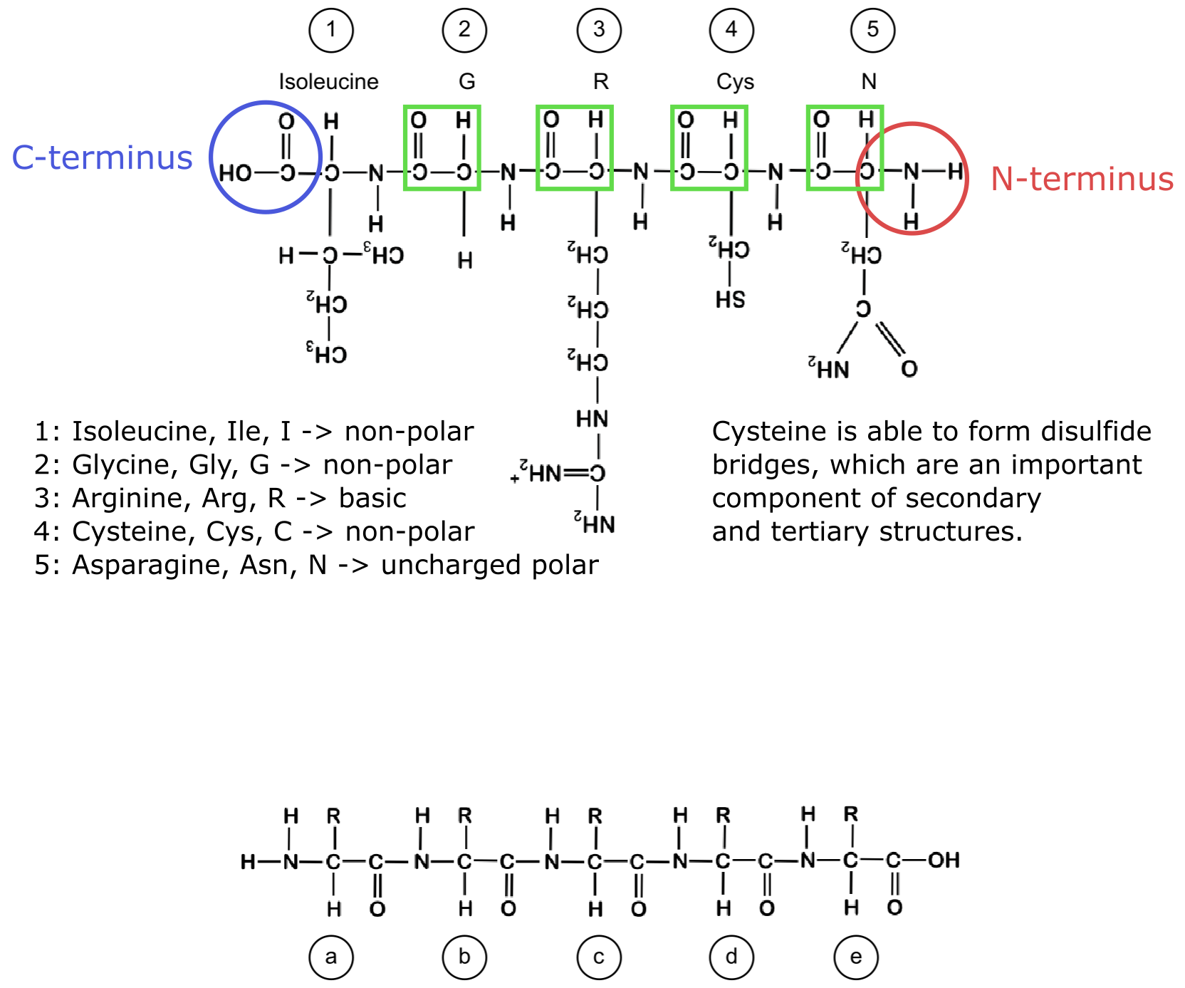
   c. Randomly distributed

6. The side chains of amino acids play important roles in the folding and the function of proteins. Below, you can see a short peptide that has been formed by five amino acids (labeled from 1 to 5).
   a. Indicate in blue and red the N-terminus and the C-terminus of the peptide, respectively, and highlight all peptide bonds in green.
   b. For each of the five amino acids (1-5), give either the name, the three-letter or the one-letter code, depending on the information lacking (for example, for amino acid 1, give the three- and the one-letter code, while for amino acid 2 give the name and the three-letter code).
   c. Indicate for each of the amino acids (1 to 5) its physiochemical properties (nonpolar, polar, acidic, basic).
   d. Describe in one sentence what specific property the side chain of amino acid 4 has, and why this property is important to form protein structures.

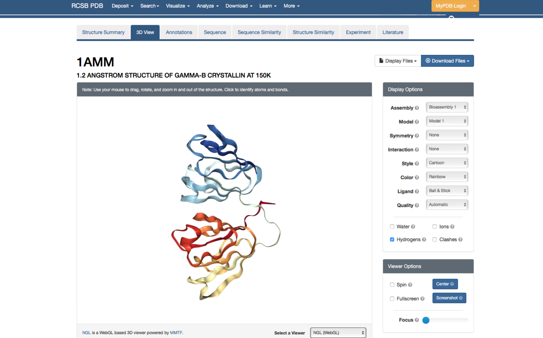
7. Amino acids and their side chains can interact with other amino acids and form bonds and interactions. Interactions between amino acids and their side chains play important roles in stable folded proteins structures. Revisit Fig. 1.15 from the reader. With this information in mind, take another look at the peptide sequence with five amino acids (see question 6). Below this peptide, you will find the backbone of another peptide in which the side chains have been only indicated with R (labeled a-e). Look at the 20 amino acids in the amino acid table in the reader. Discuss with your neighbour which of the 20 possible amino acids could be placed as a side chains R (a-e) such that these can likely interact, i.e., forms bonds or other interactions, with the corresponding amino acids (1-5) in the upper peptide (i.e., a interacts with 1, b with 2, and so on). Indicate for each which type of interaction (e.g., hydrogen bonds) are occurring between your proposed pair of amino acids. 8.Proteins fold into compact structures, and this structure is important for proteins to have biological functional activity. In folded proteins (tertiary structure), the secondary structure is often still visible, i.e., helices and beta sheets are still visible. Sometimes proteins are not only formed by a single structural unit, a so-called domain, but by multiple domains that can either be the same type or of different types. Sometimes, it can be useful to look at the tertiary structure of proteins with known fold (either experimentally or in silico determined), e.g., to see where mutations in the structure occur. We will have a look at the protein structure of Gamma B-Crystallin. Go to the website of PDB, which is a resource for protein structures, and search on the main page for Gamma B-Crystallin, with the ID “1AMM”. Click on ‘3D View’ to see a three-dimensional model of the structure. On the bottom right, change the viewer to NGL.
   a. Color the structure by Secondary structure (see ‘Color’, under ‘Structure View’). Under ‘Structure View Documentation’ you can find the meaning of each color. Can you identify the number of secondary structure elements (helix, sheet) you can observe in the structure?
   b. How many domains does this protein have?

8. Amino acid quiz: you have now worked extensively with amino acids and you should know the relation between the 1- and 3-letter code, the name of the amino acid and its biochemical properties. To test this knowledge once more, perform this small test by filling in the missing information in the table (do not look at the reader before finalizing the quiz).

	1-letter	3-letter	Full name	Class
1			Glutamic acid	Nonpolar/Polar/Acidic/Basic
2		Phe		Nonpolar/Polar/Acidic/Basic
3	T			Nonpolar/Polar/Acidic/Basic
4		Pro		Nonpolar/Polar/Acidic/Basic
5			Serine	Nonpolar/Polar/Acidic/Basic
6	K			Nonpolar/Polar/Acidic/Basic
7			Isoleucine	Nonpolar/Polar/Acidic/Basic
8		Asn		Nonpolar/Polar/Acidic/Basic
9			Methionine	Nonpolar/Polar/Acidic/Basic
10	A			Nonpolar/Polar/Acidic/Basic
11	P			Nonpolar/Polar/Acidic/Basic
12		His		Nonpolar/Polar/Acidic/Basic

Assignment II answers

1. Glycine is the smallest amino acid; it only has one hydrogen (H) atom as its side chain.

2. The nonpolar amino acids are generally hydrophobic. So, you could have listed any of glycine, alanine, valine, leucine, isoleucine, proline, phenylalanine, methionine, tryptophan, cysteine.

3. Aspartic acid and glutamic acid

4. Answer a is incorrect, A stands for Alanine

5. The nonpolar amino acids are hydrophobic (not liking water), and therefore tend to be buried inside the protein surrounded by other hydrophobic amino acids.

6. Side chain activities

7. Side chains and their activities
   a & b: other non-polar aa such as Val/Ala/Ieu -> hydrophobic
   c: Asp -> electrostatic
   d: Cys -> disulfide
   e: Tyr (or any other polar amino acid)-> hydrogen bond

8. Protein structures
   a. there are 2 times 4 and 3 large beta strands (organized in 2 anti-parallel beta-sheets). Furthermore, the structure contains 1 alpha-helix and 3 3/10 helices, the fourth most common type of protein secondary structures.
   b. Likely two identical domains. If you look under “Annotations” in the menu, you see various different annotation sources that mention a gamma-crystallin domain. Under the “Sequence” tab you can see where these domains are on the protein, for example the PFAM or SCOP annotations clearly show two domains.

9. Amino acid quiz

	1-letter	3-letter	Full name	Class
1	E	Glu	Glutamic acid	Nonpolar/Polar/Acidic/Basic
2	F	Phe	Phenylalanine	Nonpolar/Polar/Acidic/Basic
3	T	Thr	Threonine	Nonpolar/Polar/Acidic/Basic
4	P	Pro	Proline	Nonpolar/Polar/Acidic/Basic
5	S	Ser	Serine	Nonpolar/Polar/Acidic/Basic
6	K	Lys	Lysine	Nonpolar/Polar/Acidic/Basic
7	I	Ile	Isoleucine	Nonpolar/Polar/Acidic/Basic
8	N	Asn	Asparagine	Nonpolar/Polar/Acidic/Basic
9	M	Met	Methionine	Nonpolar/Polar/Acidic/Basic
10	A	Ala	Alanine	Nonpolar/Polar/Acidic/Basic
11	P	Pro	Proline	Nonpolar/Polar/Acidic/Basic
12	H	His	Histidine	Nonpolar/Polar/Acidic/Basic

\pagebreak

Assignment III: Databases (45 minutes)

1. In a web browser, navigate to the Molecular Biology Database Collection of the journal Nucleic Acids Research (NAR). Pick three databases from the list that draw your attention, preferably from different categories, and explore them (approx. 5 min each).
   a. What type of data is in there?
   b. What would it be used for? Highly specialized or broad applications?
   c. How can you search the database?
   d. Does it look up-to-date and regularly maintained?

2. Redundancy
   a. What does redundancy in a database mean? Give an example of redundancy in a sequence database.
   b. Are the UniProt databases redundant or non-redundant?
   c. What is the difference between RefSeq and GenBank in terms of redundancy?

3. Ontology
   a. Describe what an ontology is (use the information in the reader and/or Google to find information).
   b. The Gene Ontology is one of the most important ontologies in bioinformatics. Which biological domains are covered in the Gene Ontology?
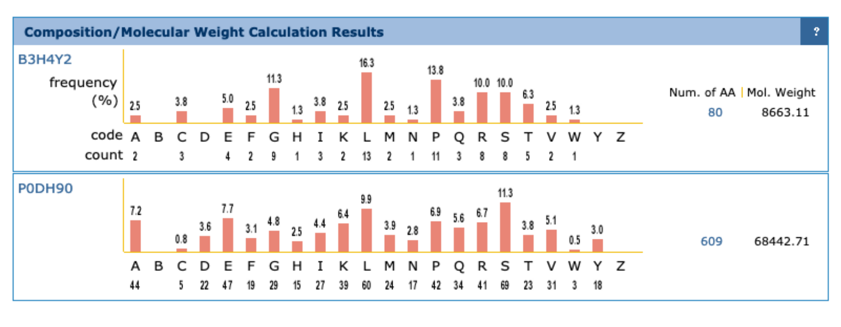
   c. Look up the Arabidopsis protein in UniProt (Accession B3H4Y2). What information do you find about the GO terms associated with this protein?
   d. Now look up the famous Arabidopsis gene FRIGIDA (Accession P0DH90). Which GO terms are associated with this gene? In which cellular component is this protein found and which biological process is it involved in?

4. UniProt
   a. Look up the two proteins from Q3 in UniProt again. In which of the sections of UniProt is each of them deposited. Which of the two has a higher annotation quality?
   b. How many publications are linked to each of these proteins? Which of these publications contains specific information on the protein (based on the title)?
   c. For each protein, look up at least one cross-reference to a database that you know and to a database that you do not yet know. Spend a few minutes to browse the information that you can gain in this way.
   d. Calculate the frequency of individual amino acids in both protein sequences using the PIR website. Do you notice something remarkable (Hint: look at relative abundance of various amino acids)? Can you relate this to information that is present in Uniprot (Hint: look at family/domains)?

5. A hot topic in biological data management is “FAIR” data. What do the letters in FAIR stand for and what do those terms mean?

Assignment III answers

1. As a result of this question you should have explored a few databases. On the exam you could be asked to mention a few databases with biological data, so it’s good to get a feeling for how much and what kind of data is out there and how the data is organized and searchable.

2. Redundancy
   a. Redundancy in a database means that the database contains multiple entries with identical data. In a sequence database it could be that a certain protein sequence of a species has been submitted by several labs.
   b. Each of the UniProt databases is non-redundant (https://www.uniprot.org/help/redundancy). Definitions of redundancy differ.
   c. GenBank is a sequence database, containing sequences submitted by individual labs or large-sequencing projects. GenBank is redundant and can be very redundant for certain loci. RefSeq is the non-redundant version of GenBank where (near-)identical entries are merged. If multiple GenBank submissions represent the same molecule for an organism, the “best” sequence is chosen to represent as the RefSeq record.

3. Ontology
   a. An ontology is a formal specification of used terms and their connections. A set of concepts and categories in a subject area or domain that shows their properties and the relations between them.
   b. Biological process, molecular function, cellular component.
   c. B3H4Y2: You find 12 annotations. There are several GO-terms assigned by UniProt, the others are assigned by arabidopsis.orh (the arabidopsis information resource). GO:0016021 suggests this is an integral component of membrane; However, the molecular function annotation are assigned through sequence similarity only (i.e., there is no experimental evidence that verifies this). The linked processes are “response to salicyclic acid, ethylene, and water deprivation” (based on expression pattern evidence).
   d. Biological processes: flower development, cell differentiation. Cellular components: nuclear speck. All terms are assigned by uniprot through ‘electronic annotation’.

4. UniProt
   a. Both proteins are in swissprot. This can be seen through the gold/silver image next to the ID at the top of the info page. From this perspective both protein annotations are equally trustworthy.
   b. B3H4Y2 is linked to 3 publications: 2 that describe the Arabidopsis genome (unspecific) and 1 (recent paper) about secreted transmembrane peptides (seems relevant). P0DH90 is linked to 8 specific publications.
   c. For B3H4Y2 it is e.g., possible to look up RefSeq, we find the genbank file of the protein. For a novel DB it is interesting to look up EnsemblPlants, which covers information on the transcript and on known variation. For P0DH90 it is also possible to look up Pfam. For a novel DB, it is interesting to look up Expression Atlas, where the expression data from several papers is presented.
   d. We find a very high fraction of Proline in B3H4Y2, this is unusual since the residue is also bound to the amino group, which has important effects on the protein structure. The proline-rich C-terminus is also noted in Uniprot (under Compositional bias).

5. 
   Findable: data is well annotated, persistent identifiers, indexed.
   Accessible: standardized communication protocols.
   Interoperable: allow linking/exchange/import of data from different sources through accepted data representations and ontologies.
   Reusable: others should be able to use it, clear, standardized descriptions, proper license, etc.

\pagebreak

Assignment IV: Genome annotation (120 minutes)

1. Explain how homology searches can be useful in genome annotation and why it is more complex for eukaryotes than for prokaryotes.

2. How does RNA-sequencing data help gene prediction? Is RNA-sequencing data on its own sufficient to annotate a genome?

3. In the UniProt databse look up the Arabidopsis protein with identifier B3H4Y2. The corresponding gene ID is AT1G65484. In a second tab, look up this gene in TAIR JBrowse. The sequence of this gene can be found on BrightSpace. In a third tab, go to the NCBI Open Reading Frame Finder and paste in the gene sequence in FASTA format and hit submit.
   a. How many ORFs are found? Are they all in the same reading frame?
   b. Do any of the ORFs correspond to the ORF in the annotated gene? Why or why not?
   c. When is a simple ORF detection tool useful? When is it insufficient?

4. Yeast (Saccharomyces cerevisiae) is a well-studied model organism. A lot of information about yeast is stored in the Saccharomyces Genome Database (SGD). You will work on the reference strain S288C. The relatively small genome of yeast gives us the opportunity to explore some online genome annotation tools (within reasonable time) and compare our findings to the high-quality annotation that is available. In the menu on SGD click on Sequence -> Reference Genome -> Genome Snapshot. Under “Features by Type” explore both the graph and the table view.
   a. How many genes does the yeast genome contain?
   b. How many tRNAs have been annotated on chromosome 3 and how many on the mitochondrial genome?
   First you will annotate the mitochondrial genome of yeast, using MITOS2.
   c. Use the mitochondrial genome, provided on Brightspace or download the sequence from SGD. What is the length of the mitochondrial (MT) genome? Be creative or use Google to find the answer. Is the MT genome linear or circular?
   d. The yeast MT genome does not use the Standard Genetic Code. Which one does it use? Use NCBI Genetic Codes to find the answer. How many codons have a different meaning?
   e. Go to MITOS2 tool. Select a relevant Reference and Genetic Code for yeast and upload the fasta file. Make sure to change the output to GFF. Hit submit. This annotation can take about 10 minutes, so continue with the next exercises (5 and 6) until the results are done.
   f. Browse the results by clicking around. How many tRNAs are predicted?
   g. Look up the first predicted tRNA in the genome browser on SGD. Does the prediction match the known tRNA? To which amino acid does this tRNA correspond? How many GO terms are associated with this tRNA gene?
   h. What can you find out about the “giy” gene? In the FAA fasta text file (download from the menu on the left) you can find the protein sequence produced by the gene. Go to InterPro and use the protein sequence to search for known protein domains/functions using InterProScan. What functional information do you find for this protein? (Running InteProScan can take a few minutes, in the meantime continue with the next question).

5. Next, we will predict protein-coding genes on chromosome 3 using the widely used Augustus ab-initio gene predictor. Augustus outputs its predictions in the GFF3 text-based file format. To be able to make sense of the Augustus output, familiarize yourself with this format here. The Augustus gene predictor has already been trained on many organisms.
   a. Upload the sequence of chromosome 3, choose the right Organism and “run AUGUSTUS” (predict genes on both strands). How many genes are predicted? How many of those contain an intron?
   b. What can you say about the function, domains, etc. of gene g100? Which databases did you use to find this information?

6. You have now seen several examples of tools used in genome annotation. Describe structural and functional genome annotation in your own words and give an example of each.

Assignment IV answers

1. Many annotated prokaryotic genomes are present in databases. For a novel genome, you can search against these databases (either nucleotide sequences of genes or protein sequences) to see if these genes/proteins are also present in this novel genome. Typically more than 50% of the genes can be identified this way. For eukaryotes this is much more complex because of introns. There it is more useful to align known proteins to a novel genome as evidence.

2. RNA-seq is a direct read-out of transcription and as such is very useful in finding splice-sites. Not all genes are always expressed, so typically RNA-seq is not sufficient to identify all protein-coding genes.

3. 
   a. 6 ORFs are detected, the reading frames are different (1, 1, 2, 2, 2, 3). Note: if you copied the gene sequence from TAIR on arabidopsis.org, you will likely have found 6 ORFs in frames 1, 1, 2, 2, 2, 2. No, because the gene contains an intron, so there’s not 1 continuous ORF in the gene sequence. After splicing, the ORF should be in the coding sequence (CDS).
   b. ORF1 corresponds to the start of the gene, but it is too long. The gene has an intron at some point, which is not translated.
   >lcl|ORF1
   MGLKMSSNALLLSLFLLLLCLFSEIGGSETTHWKIGQCLPISH
   NSSSYQWIFFSPKPNLAYLRIWLFLETNYNRRISNSALFLLLLYCIK
   The first CDS has a length of 106 (producing 35 AAa), the second part 137, together 243. The second part of the protein does not start with a start codon, so it won’t be found by ORFFINDER.
   c. In prokaryotes, when there are no introns in the genes, it is very useful. In eukaryotes containing many genes with introns, it typically does not work.

4. 
   a. 6572 protein-coding genes.
   b. 10 tRNAs on Chr 3, 24 on mt.
   c. 85,779 nt (85.8 Kb), circular genome.
   d. https://www.ncbi.nlm.nih.gov/Taxonomy/Utils/wprintgc.cgi#SG3. 6 codons have a different meaning. https://en.wikipedia.org/wiki/Yeast_mitochondrial_code also mentions that 2 codons are absent.
   e. Select chrmt.fasta as the fasta file, Yeast(3) as the genetic code and RefSeq63 Metazoa as your reference data.
   f. When you look in the GFF file, you can count 24 tRNAs.
   g. Yes: the coordinates of the first tRNA match the reference annotation (but for example in the second one the stop position is different, so the coordinates do not always match). The tRNA corresponds to Proline, 3 GO terms: GO:0005739, GO:0006414, GO:0030533.
   h. The protein seems to be some sort of polymerase according to for example the ‘homologous superfamily’ section of the output. Associated GO term: mRNA processing (GO:0006397).

5. 
   a. 143 predicted, 9 with an intron (search for the word intron, look at them and count).
   b. Using InterProScan, the information you find is limited, for example there are no associated GO terms. There is a domain of an ATP-dependent chromatin-remodelling protein, which could provide hints for further research into this proteins function. If you used BLASTP on UniProt, you could have found a lot more information: it seems this protein is RSC6_YEAST, and there is for example some literature on this class of proteins. NOTE: using BLASTP was not part of this week’s assignment, so you are not expected to have found this information at this point in the course. \

6. Structural annotation is the identification of genome features in the genome, e.g., start and stop positions of gene regions, exons, introns, UTRs, CDS. Functional annotation is assigning biological information to the genome features, e.g., protein function, domains, enzyme codes, type of transposon, etc.

\pagebreak

Project Preparation Exercise

We want to obtain insights into members of the ARF gene family in Arabidopsis thaliana. ARF5 (UniProt ID P93024) and IAA5 (UniProt ID P33078) are two well-studied A. thaliana proteins that play a role in auxin-mediated regulation of gene expression. They are therefore chosen here as the starting points for exploring the plant ARF gene family. Perform a small background study on ARF5 and IAA5. Explore the protein sequences, properties (e.g., length, composition, etc.), interaction partners, and functional regions of ARF5 and IAA5. Finally, explore the genes encoding ARF5 and IAA5 in A. thaliana (genomic location, exon structure, expression, etc.).

Describe the following items in a few bullet points each. You may include up to two figures or tables.

1. Materials & Methods What did you do? Which data, databases and tools did you use, and why did you choose these? What important settings did you select?

2. Results What did you find, what are the main results? Report the relevant data, numbers, tables/figures, and clearly describe your observations.

3. Discussion & Conclusion Do the results make sense? Are they according to your expectation or do you see something surprising? What do the results mean, how can you interpret them? Do different tools agree or not? What can you conclude? Make sure to describe the expectations and assumptions underlying your interpretation.

References

1W1

Mary Ann Clark, Matthew Douglas, and Jung Choi. 3.5 Nucleic Acids. OpenStax, Houston, Texas, 2018. URL: https://openstax.org/books/biology-2e/pages/3-5-nucleic-acids.

1W2

OpenStax College. Dna nucleotides. 2013. URL: https://commons.wikimedia.org/wiki/File:DNA_Nucleotides.jpg.

1W3

Madeleine Price Ball. Dna replication split. 2013. URL: https://commons.wikimedia.org/wiki/File:DNA_replication_split.svg.

1W4

Lizanne Koch. Semiconservative replication. 2009. URL: https://commons.wikimedia.org/wiki/File:Semiconservative_replication.png.

1W5

UC Museum of Paleontology. The causes of mutations. 2020. URL: https://evolution.berkeley.edu/evolution-101/mechanisms-the-processes-of-evolution/the-causes-of-mutations/.

1W6(1,2,3,4,5,6,7,8)

Dick de Ridder, Anne Kupczok, Rens Holmer, Freek Bakker, Justin van der Hooft, Judith Risse, Jorge Navarro, and Tomer Sardjoe. Self-created figure. 2024.

1W7

miguelferig. Intron miguelferig. 2011. URL: https://commons.wikimedia.org/wiki/File:Intron_miguelferig.jpg.

1W8

Sarah Greenwood. Genetic code. 2018. URL: https://commons.wikimedia.org/wiki/File:Genetic_Code.png.

1W9

Squidonius. Molbio-header. 2008. URL: https://commons.wikimedia.org/wiki/File:Molbio-Header.svg.

1W10(1,2,3)

Mary Ann Clark, Matthew Douglas, and Jung Choi. 3.4 Proteins. OpenStax, Houston, Texas, 2018. URL: https://openstax.org/books/biology-2e/pages/3-4-proteins.

1W11

LadyofHats. Main protein structure levels en. 2008. URL: https://commons.wikimedia.org/wiki/File:Main_protein_structure_levels_en.svg.

1W12

OpenStax College. Protein structure. URL: https://openstax.org/books/microbiology/pages/7-4-proteins#OSC_Microbio_07_04_secondary.

1W13

R. A. Laskowski, M. W. MacArthur, D. S. Moss, and J. M. Thornton. Procheck: a program to check the stereochemical quality of protein structures. Journal of Applied Crystallography, 26(2):283–291, 1993. URL: https://onlinelibrary.wiley.com/doi/abs/10.1107/S0021889892009944, arXiv:https://onlinelibrary.wiley.com/doi/pdf/10.1107/S0021889892009944, doi:https://doi.org/10.1107/S0021889892009944.

1W14

Amaia Sangrador. What are protein domains? 2023. URL: https://www.ebi.ac.uk/training/online/courses/protein-classification-intro-ebi-resources/protein-classification/what-are-protein-domains/.

1W15(1,2,3)

H.M. Berman, J. Westbrook, Z. Feng, G. Gilliland, T.N. Bhat, H. Weissig, I.N. Shindyalov, and P.E. Bourne. The protein data bank. 2000. URL: http://www.rcsb.org/, doi:10.1093/nar/28.1.235.

1W16

Y. Liang, Z. Hua, X. Liang, Q. Xu, and G. Lu. Crystal structure analysis of bar-head goose hemoglobin (deoxy form). 2001. URL: http://doi.org/10.2210/pdb1hv4/pdb, doi:10.1006/jmbi.2001.5028.

1W17(1,2,3)

A.S. Rose, A.R. Bradley, Y. Valasatava, Duarte J.M., A. Prlić, and P.W. Rose. Ngl viewer. 2018. NGL viewer: web-based molecular graphics for large complexes. doi:10.1093/bioinformatics/bty419.

1W18

J.B. Thoden, T.M. Wohlers, J.L. Fridovich-Keil, and H.M. Holden. Structure of human udp-galactose 4-epimerase in complex with nad+. 2000. URL: http://doi.org/10.2210/pdb1ek5/pdb, doi:10.1021/bi000215l.

1W19

J.B. Cooper, G. Khan, G. Taylor, I.J. Tickle, and T.L. Blundell. X-ray analyses of aspartic proteases. ii. three-dimensional structure of the hexagonal crystal form of porcine pepsin at 2.3 angstroms resolution. 1990. URL: http://doi.org/10.2210/pdb5pep/pdb, doi:10.1016/0022-2836(90)90156-G.

1W20

R. Buels, E. Yao, C.M. Diesh, R.D. Hayes, M. Munoz-Torres, G. Helt, D.M. Goodstein, C.G. Elsik, S.E. Lewis, L. Stein, and I.H. Holmes. Jbrowse: a dynamic web platform for genome visualization and analysis. Genome Biology, 2016. doi:10.1186/s13059-016-0924-1.

1W21

D.A. Benson, M. Cavanaugh, K. Clark, I. Karsch-Mizrachi, D.J. Lipman, J. Ostell, and E.W. Sayers. Genbank. Nucleic Acids Research, 41(D1):D36–D42, 2012. doi:10.1093/nar/gks1195.

1W22

A. Leon and O. Pastor. Towards a shared, conceptual model-based understanding of proteins and their interactions. IEEE Access, 9:73608–73623, 2021. doi:10.1109/ACCESS.2021.3080040.

1W23(1,2,3,4)

T. Paysan-Lafosse, M. Blum, S. Chuguransky, T. Grego, B.L. Pinto, G.A. Salazar, M.L. Bileschi, P. Bork, A. Bridge, L. Colwell, J. Gough, D.H. Haft, I. Letunić, A. Marchler-Bauer, H. Mi, D.A. Natale, C.A. Orengo, A.P. Pandurangan, C Rivoire, C.J.A. Sigrist, I. Sillitoe, N. Thanki, P.D. Thomas, S.C.E. Tosatto, C.H. Wu, and A. Bateman. Interpro in 2022. Nucleic Acids Research, 51(D1):D418–D427, 2022. doi:10.1093/nar/gkac993.

1W24

Alex Mitchell. Interpro entry types. 2020. URL: https://en.m.wikipedia.org/wiki/File:InterPro_Entry_types.png.

1W25

D. Binns, E. Dimmer, R. Huntley, D. Barrell, C. O'Donovan, and R. Apweiler. Quickgo: a web-based tool for gene ontology searching. Bioinformatics, 25(22):3045–6, 2009. doi:10.1093/bioinformatics/btp536.

1W26

K. Eilbeck, S.E. Lewis, C.J. Mungall, M. Yandell, L. Stein, R. Durbin, and M. Ashburner. The sequence ontology: a tool for the unification of genome annotations. Genome Biology, 2005. doi:10.1186/gb-2005-6-5-r44.