
2. Alignment, sequence search, and primer design#
– Anne Kupczok, Rens Holmer
In chapter 2 of Introduction to Bioinformatics, you will study sequence alignment.
Make sure you understand what DNA and protein alignments are used for and that you can explain the differences between local and global alignments. You should be familiar with concepts related to alignments and sequence search, like dotplots, alignment scores, e-values, and substitution matrices. Make sure you understand what multiple alignments are used for and that you can explain the differences between different solutions for the MSA problem. You should understand what motifs are and the basics of profile hidden Markov models. This chapter concludes with a section on PCR primer design as an example on the use of sequence alignment algorithms in practice.
During the practical you will learn how to make pairwise and multiple-sequence alignments, perform sequence searches and motif analyses, design primers, and discuss the results.
Introduction#
Comparing DNA and protein sequences is a key tool in the field of applied bioinformatics. By analyzing these sequences, researchers can annotate genes from new genomes, build models of protein structures, and investigate gene expression, i.e., which genes are turned on and off. It is important to notice that nature tends to stick with what works, rather than reinventing the wheel for each species. Instead, organisms evolve from ancestors, they accumulate mutations (Chapter 1), and gradually develop new traits over time. That means that similar genes can be found in different organisms and the functional information can be transferred from one protein to another if both possess a certain degree of similarity. However, even though two proteins may look similar, they could also have different functions. Generally, similarities arise because of shared ancestry (divergent evolution), nevertheless, similarities can also appear independently (convergent evolution).
Before diving into the analysis of whether sequences are related, it is important to understand some key terms.
Homology and similarity
Homology means that sequences share a common evolutionary history and therefore have a common ancestor. Homology is not quantifiable. If two sequences have a common ancestor, they are homologous. Thus, two sequences are either homologous or they are not.
Sequence identity and sequence similarity are often used to infer whether two sequences are homologous. We can measure the identity or similarity between sequences and we will see how to do this later in this chapter.
In contrast, we cannot measure homology, but we can only infer it.
See also
Here is a classic paper on homologous protein families: Tatusov et al., 1997.
Dot plots#
Dot plots are a simple way to visualize similar regions between two sequences. They are represented by a two-dimensional array, where one sequence is written vertically and the other horizontally. A dot is placed in a cell, where the residues are identical. In the resulting plot, similar regions appear as diagonal stretches and insertions and deletions appear as a discontinuity in a diagonal line (Fig. 2.1).
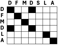
Fig. 2.1 A small example of a dotplot.
Credits: CC BY-NC 4.0 [Ridder et al., 2024].#
A sequence can also be compared to itself, then the main diagonal will be filled with dots and additional repeats are on the off-diagonal (Fig. 2.2).
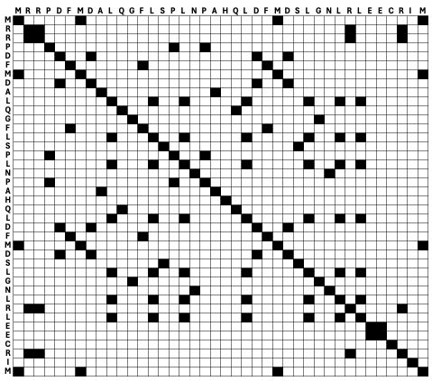
Fig. 2.2 An example of a dotplot to compare a sequence with itself. Credits: CC BY-NC 4.0 [Ridder et al., 2024].#
This simple way of marking identical residues shows a lot of background noise. To detect interesting patterns, typically a filter is applied. For example, a minimum identity should be present across a certain window size, i.e., consecutive number of residues being considered. This feature is implemented in a webserver to visualize dotplots, dotlet [Junier and Pagni, 2000] (Fig. 2.3).
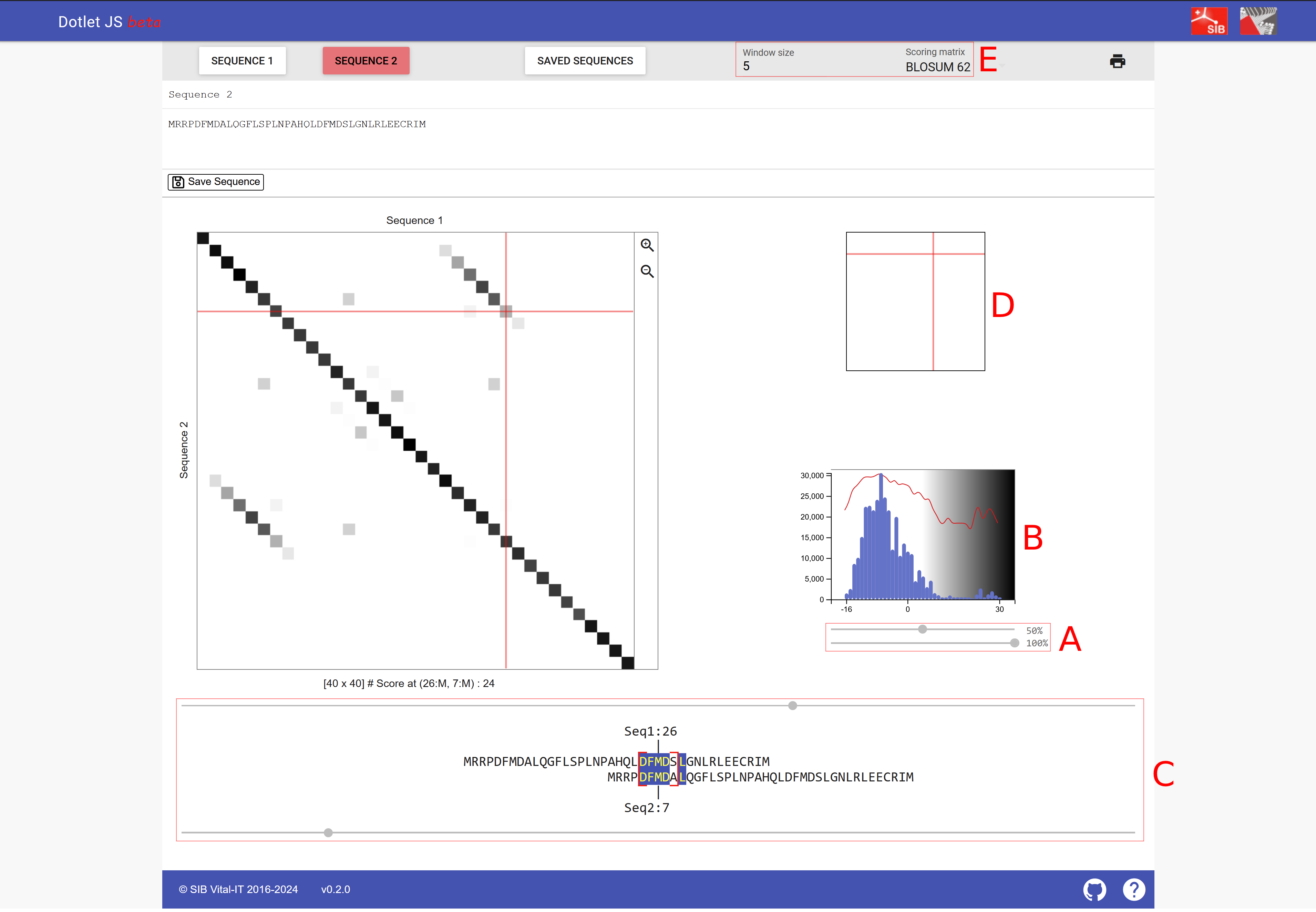
Fig. 2.3 A screenshot of dotlet with sequence MRRPDFMDALQGFLSPLNPAHQLDFMDSLGNLRLEECRIM.#
(A) The two sliders to change the appearence of the plot: The top slider can adjust the sensitivity, moving it to the right, fewer similar regions are shown; moving it to the left, also regions with lower similarity appear. The bottom slider adjusts the color scheme and is less relevant compared to the top slider.
(B) The histogram indicates how many hits with a particular similarity are shown; thus the slider can be adjusted to the right tail of the histogram.
(C) The two sliders that can adjust how the two sequences are positioned against each other.
(D) Serves a similar function as the two sliders of C but allows for arrow key navigation of the dotplot.
(E) Here you can select the window size of sequence comparison and the scoring matrix (window size is explained below and substitution matrices will also be explained below).
Credits: [Junier and Pagni, 2000].
Pairwise alignment#
Dot plots provide a visual way to compare two sequences, however, they do not provide the similarity between two sequences. To calculate sequence similarity or sequence identity, we need to perform a pairwise sequence alignment. In an alignment, the two sequences will be placed above each other and gaps can be introduced to represent insertions or deletions of residues. We also say that the two sequences will be aligned. The resulting alignment contains matches, mismatches, and gaps (Fig. 2.4)

Fig. 2.4 A small example of two aligned sequences. Credits: CC BY-NC 4.0 [Ridder et al., 2024].#
Alignments of DNA sequences#
Every position in a sequence could potentially have an instertion or a deletion, so there are many possible locations and combinations for gaps and thus many potential alignments. The final alignment will be the one with the maximum total alignment score. This score is determined by the scoring parameters that are chosen before the alignment calculation. An example of DNA sequence scoring paramaters could be that matches score 1 and mismatches -1 and that there is a gap penalty of -1. The total alignment score is calculated by summing over all columns in the alignment (Fig. 2.5).
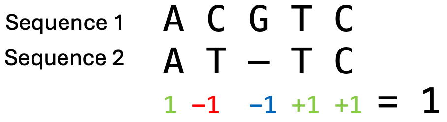
Fig. 2.5 An example calculation of the alignment score, where matches score 1, mismatches -1 and there is a gap penalty of -1. This results in a total score of 1 for this alignment. Credits: CC BY-NC 4.0 [Ridder et al., 2024].#
The choice of the scoring parameters has an impact which alignment will have the maximum score. To understand the impact of the parameters on the final alignment, fill in table Fig. 2.6.

Fig. 2.6 Assignment: Fill the table for the two alignments and the two sets of scoring parameters. Credits: CC BY-NC 4.0 [Ridder et al., 2024].#
Note 2.1: Affine gap costs
The DNA and protein sequences that we want to align often have varying lengths, which is the result of insertions and deletions during evolution. Insertion and deletion events can affect one or multiple residues, where one event of length 2 is more likely to happen than two independent events of length 1. To include this in the scoring scheme, alignment programms use affine gap costs that distinguish between opening a gap and extending a gap. For example, the default parameters of the pairwise alignment program needle [Madeira et al., 2022] are:
Gap open (score for the first residue in a gap): -10
Gap extend (score for each additional residue in a gap): -0.5
Alignments of protein sequences#
Substitution matrices#
In chapter 1, we learned that different amino acids have different chemical properties. When the protein structure and function are conserved, it is more likely that an amino acid gets exchanged by a chemically similar amino acid, compared to a very different one. When aligning protein sequences, we thus want to penalize the exchange of chemically dissimilar amino acids and reward the exchange of chemically similar amino acids. To this end, the score of matches and mismatches is generally determined by a substitution matrix, e.g., BLOSUM62 - BLOSUM (BLOck SUbstitution Matrix) (Fig. 2.7). The substitution matrix and the gap parameters then determine the alignment score (Fig. 2.8).

Fig. 2.7 The BLOSUM62 amino acid substitution matrix. The matrix is ordered and positive values and zero values are highlighted. Credits: CC BY-SA 4.0 [Ppgardne, 2022].#
Box 2.1: Assignment
Look at the amino acid properties in the table in chapter 1, choose some amino acids with the same properties and some with different properties. Then look up these pairs in the BLOSUM62 matrix. What do you observe?
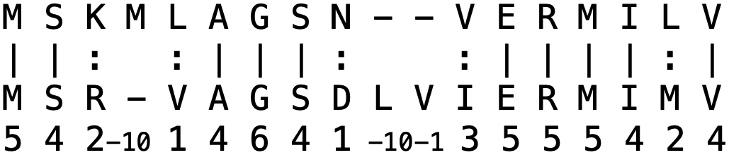
Fig. 2.8 Example of a pairwise protein alignment. With the BLOSUM62 scoring matrix, a gap opening score of -10, and a gap extension score of -1, the resulting alignment score is 34. Credits: CC BY-NC 4.0 [Ridder et al., 2024].#
Note that we motivated the use of amino acid substitution matrices by the chemical properties of amino acids; however, these properties were not directly used when determining these matrices. Instead, the BLOSUM matrix is determined by aligning conserved regions from Swiss-Prot (chapter 1) and clustering them based on identity. Then, the substitutions between the different pairs of amino acids within a cluster are counted, which is used to compute the BLOSUM scores. Thus, these scores reflect directly which amino acids are exchanged more often with each other over evolutionary time and we can observe that this frequency is strongly correlated to their chemical properties. There are different versions of BLOSUM, for example BLOSUM62 was derived by clustering sequences with an identity of 62% and it is appropriate for comparing protein sequences having around 62% identity. Other available matrices are for example BLOSUM45 and BLOSUM80 (Fig. 2.9).
Another group of matrices that was derived even before BLOSUM is PAM (Point Accepted Mutation). The entries in a PAM matrix denote the substitution probabilities of amino acids over a defined unit of evolutionary change. For example, PAM1 represents one substitution per 100 amino acid residues and is thus appropriate for very closely related sequences. A commonly used matrix is PAM250, which means that 250 mutations happened over 100 residues; that is, many residues have been affected by more than one mutation.

Fig. 2.9 An overview of different available substitution matrices. Credits: CC BY-NC 4.0 [Ridder et al., 2024].#
See also
An introduction into PAM and BLOSUM substitution matrices.
Protein identity and similarity#
For two protein sequences, we can distinguish two different measures of how much they are alike: identity and similarity, which are defined slightly differently. The protein identity is given by the number of identical amino acids divided by the alignment length. The protein similarity is given by the number of similar amino acids and the number of identical amino acids divided by the alignment length. In the pairwise alignment program needle, identical amino acids are marked by a pipe symbol/vertical line (|), similar amino acids are marked by a colon (:) and defined by pairs that have a positive score (i.e., >0) in the chosen substitution matrix (Fig. 2.10).
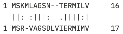
Fig. 2.10 Example protein alignment. The percent identity is 10 / 18 = 55.6% and the percent similarity is 14 / 18 = 77.8%. Credits: CC BY-NC 4.0 [Ridder et al., 2024].#
Note that the pairwise alignment method does not try to maximize similarity or identity, but they are a result of the chosen parameters. Especially for distantly related sequences, the parameters can have a big impact on the alignment and thus on the estimated identity and similarity. In Fig. 2.11, you can find an example of two protein kinases from rice.
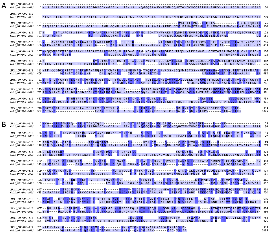
Fig. 2.11 Alignments of the same two sequences (LERK1_ORYSI and XA21_ORYSI) with different parameters: A) BLOSUM62 matrix, gap open: -10, gap extend: -0.5. Identity = 210/1191 (17.6%), Similarity = 345/1191 (29.0%). B) BLOSUM62 matrix, gap open: -5, gap extend: -0.5. Identity = 305/1166 (26.2%), Similarity = 428/1166 (36.7%). Credits: CC BY-NC 4.0 [Ridder et al., 2024] made using needle [Madeira et al., 2022].#
Up until now, we have only considered pairwise alignments, where both sequences are aligned completely, these are called global alignments.
Note 2.2: Finding the best alignment
There is a huge number of alignments possible for two sequences, since the gaps can be placed in many different ways. However, to find the optimal alignment, i.e., the one with the highest score, it is not necessary to explore all these possibilities. Efficient algorithms exist that guarantee to find the optimal alignment. The Needleman-Wunsch algorithm was the first algorithm and can solve this task in a time that is quadratic to the length of the input sequences.
Local alignments#
The previous example shows that some sequences might not be related over their full length. We have seen in chapter 1 that many proteins are composed of domains. When comparing two proteins, only some parts that correspond to the domains might be related. Then, it is more appropriate to perform a local alignment. Local alignment is also a good tool for identifying functional sites from which sequence patterns and motifs can be derived Fig. 2.12.
The aim of a local alignment is to find the best subsequences of both input sequences that result in the maximum alignment score given the alignment parameters. As for global alignment, efficient algorithms exist to solve this task. The Smith-Waterman algorithm can also solve this task in a time that is quadratic in the length of the input sequences, just like the Needleman-Wunsch algorithm for global alignments.
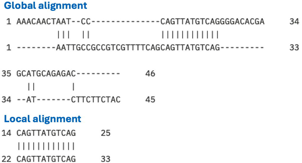
Fig. 2.12 Alignments of the same two sequences, once using the global alignment program needle and once using the local alignment program water [Madeira et al., 2022]. The same alignment paramters were used: DNAfull matrix, gap open -10, gap extend -0.5. The global identity is 20/71 (28.2%) and the local identity is 12/12 (100.0%). Credits: CC BY-NC 4.0 [Ridder et al., 2024].#
Search in sequence databases#
In Chapter 1, we learned about different sequence databases. We often want to search novel sequences in these databases, for example to learn which other organisms have homologs. Two sequences that are highly similar, might also share the same function. This relationship is used for the functional annotation of sequences, where the search in databases is an important step.
Note 2.3: Similarity by chance
When all nucleotides occur randomly and at the same frequency, then each sequence of length x is expected to occur with a frequency of 1/4x, e.g., a sequence of length 3 has a frequency of 1/64 and a sequence of length 10 has a frequency of about 1 in a million.
This becomes important since these days, databases are very large, they can contain millions of sequences.
Due to this large amount of data, some similarities might just be observed by chance, especially if our sequence of interest is short.
Thus, statistical methods have been developed to estimate if an observed alignment might have just occured due to chance (see below).
Database search vs. pairwise alignment#
Pairwise alignments are also used when searching sequences in sequence databases. In this task, we have a query sequence and we want to find similar sequences in a database; these similar sequences are called subjects or hits. Although the algorithms that were discussed in the previous section are relatively fast when two sequences are aligned, it would still take too long overall to perform pairwise sequence alignments of the query with all potential subjects from the database. We thus need even more efficient algorithms.
Note 2.4: Heuristic algorithms
The Needleman-Wunsch and the Smith-Waterman algorithm described in the previous section guarantee to find the alignment with the best score for the given sequences and parameters. In contrast, an heuristic algorithm employs some heuristics, which generally lead to good results and which make the algorithm much faster. However, the method does not guarantee to find the optimal score anymore.
BLAST#
Basic Local Alignment Search Tool (BLAST) is a heuristic method to find regions of local similarity between protein or nucleotide sequences. The program compares nucleotide or protein sequences to sequences in a database and calculates the statistical significance of the matches. Both the standalone and web version of BLAST are available from the National Center for Biotechnology Information (NCBI).
The algorithm#
The starting point of BLAST is the set of words that two sequences have in common, where a word is a part of a sequence of a fixed length. For protein blast, the default word size is 5 and for nucleotide blast it is 11. To find these common words, first a lookup table of the query words is reconstructed (Fig. 2.13A), where neighborhood words are listed as well. Neighborhood words are all the words that have a high alignment score with the query word (Fig. 2.13B). Then, BLAST scans the database for word matches. For protein blast, two matches within 40 residues must be found such that the BLAST considers the hit as an initial match (Fig. 2.13C). Note that for nucleotides, initial hits are found in a simpler way: Only one exact match must be found, i.e., no neighborhood is considered.
After finding initial matches, BLAST extends these matches into local alignments (Fig. 2.13D). As this extension happens, the alignment score increases or decreases. When the alignment score drops below a set level, the extension stops. This prevents the alignment from stretching into areas where there is very little similarity between the query and hit sequences. If the obtained alignment receives a score above a certain threshold, it will be included in the final BLAST result. BLAST is thus a heuristic algorithm, but its careful process helps to ensure a reasonable trade-off between run time and accuracy.

Fig. 2.13 An overview of the BLAST algorithm. Credits: CC0 1.0 [National Library of Medicine (NLM), 2022].#
BLAST output#
The BLAST output contains vast information on the found hits, their alignments, and taxonomy (Fig. 2.14).
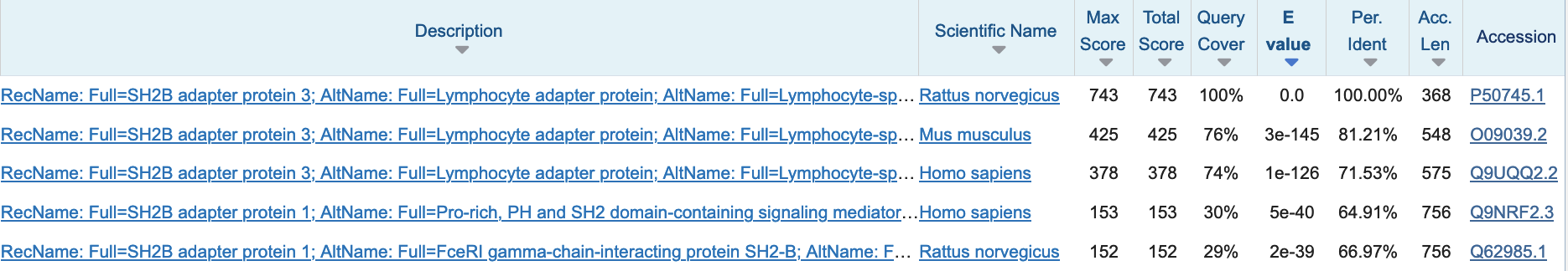
Fig. 2.14 Top 5 blast hits when searching the rat protein P50745 in the Swiss-Prot 2024_02 release database. Credits: [Camacho et al., 2009]#
Note 2.5: E-value
An important output statistic is the expectation value (e-value), which is the number of BLAST hits you expect to see by chance in the database, with the observed score or higher. Note that due to this definition, the e-value depends on the database size. Since it is more likely to find something by chance in a larger database, the e-value for the same hit would be higher compared to a smaller database. Thus, to find as many good hits as possible, it makes sense to use the smallest specific database that contains all the sequences you are interested in. For example, if you are only interested in plants, then restrict your search to only plant sequences. During the practical you will get to know how to do that in the online BLAST interface.
The BLAST output is sorted by increasing e-value. This can result in very low numbers and the BLAST output uses the scientific notation to list these, where e.g., 3e-145 means 3*10-145. Thus, the hits listed in Fig. 2.14 are likely not random, since their number to be observed by chance is very low. If the alignment is not by chance, then it might be due to a biological meaningful relationship between the two sequences. However, it is difficult to define a clear e-value cutoff for biologically meaningful hits. Commonly used cutoffs are 1e-5 or 1e-10.
Note that you cannot infer homology by e-value alone, also the coverage and percent identity need to be taken into account. For example, in Fig. 2.14, all hits have very low e-value: the first hit is to the sequence itself, then there are hits with high identity and high coverage in mouse and human, these might be homologous sequences. The 4th and 5th hit are only local, since the query cover is ~30%, these sequences might only share a homologous domain with the query protein.
BLAST types#
Different types of BLAST exist to search nucleotides or proteins in the respective databases:
blastn searches a nucleotide sequence in a nucleotide database and blastp searches a protein sequence in a protein database.
In addition, the query and/or the database can also be translated in all six reading frames to allow additional kinds of comparisons (Fig. 2.15).
Different BLAST types exist for these different kinds of comparisons, where these translations are done automatically (Fig. 2.15).

Fig. 2.15 Different BLAST types to compare different data types. Credits: CC BY-NC 4.0 [Ridder et al., 2024].#
Multiple sequence alignment#
One straightforward observation from a sequence search is that one query sequence often has multiple similar sequences (Fig. 2.14). This can lead to research questions on for example evolution (where do these sequences come from?), function (why are some sequences more similar to each other than to others?), or structure (are all parts of these sequences equally similar/dissimilar?). To compare all of these sequences with each other using a pairwise alignment strategy would quickly lead to a large number of comparisons and would be difficult to interpret. Instead, in cases where we want to compare 3 or more sequences with each other, we turn to multiple sequence alignment.
The objective of performing multiple sequence alignment is to identify matching residues (DNA, RNA, or amino acids) across multiple sequences of potentially differing lengths. Similar to pairwise alignment, the result is called ‘a multiple sequence alignment’. The resulting multiple sequence alignment can be thought of as a square matrix: rows represent the sequences that we started with, columns represent homologous residues across sequences, and the entries are either residues or gaps (Fig. 2.16).

Fig. 2.16 Conceptual diagram depicting multiple sequence alignment. Colored dots represent similar sequence elements, in the multiple sequence diagram on the right these elements align in vertical columns. Credits: CC BY-NC 4.0 [Ridder et al., 2024].#
Various algorithms for creating multiple sequence alignments exist. Here we will go over two main concepts that are adopted by many tools: progressive alignment and iterative alignment.
Progressive alignment#
To avoid having to reconcile many pairwise alignments, progressive alignment takes an iterative approach using a guide tree. The guide tree represents a crude measure of similarity between all sequences that are to be analyzed. Progressive alignment picks the two most similar sequences using the guide tree and initializes the multiple sequence alignment by aligning these two sequences with a global alignment strategy. Subsequently, the guide tree is used to determine the order in which sequences are added to the alignment. One way of thinking about this, is that progressive alignment creates increasingly large ‘blocks’ of sequences, where a block is always treated as a unit (e.g. introducing a gap will happen for all sequences in the block). By iterating through the guide tree, this alignment strategy ‘progresses’ to the final result, hence the name ‘progressive alignment’.
Box 2.2: Constructing a guide tree
The guide tree that is used by the progressive alignment strategy is typically created with a clustering algorithm that takes as input all pairwise distances between sequences. Obtaining these pairwise distances can be done through e.g. local alignment scores, but another common approach is to count the number of subsequences of length \(K\) (also known as k-mers) that are present in both sequences of a sequence pair. The downside of this k-mer based strategy is that it provides a crude distance measure (and is therefore not very accurate), the benefit is that it is very fast.
In addition, once a multiple sequence alignment has been created with the progressive strategy, it is straightforward to recompute the guide tree based on this first multiple sequence alignment and calculate a second multiple sequence alignment based on this updated guide tree. This recomputing of the guide tree could in theory be repeated infinitely many times, in practice it seems sufficient to only recompute once. The often used multiple sequence alignment program mafft implements recomputing the guide tree in the FFT-NS-2 algorithm.
Iterative refinement#
One potential downside of the progressive alignment strategy is that some of the intermediate blocks represent sub-optimal alignments. For example, when a gap is introduced during an early stage of the progressive approach, it is never removed from the alignment. Identifying and potentially improving such cases is often referred to as ‘iterative refinement’ and typically happens on a multiple sequence alignment that was created with a progressive strategy.
Iterative refinement takes as input a multiple sequence alignment, a scoring function for the multiple sequence alignment, and a function to rearrange the multiple sequence alignment. It produces a ‘refined’ multiple sequence alignment by rearranging the multiple sequence alignment and only keeps the new multiple sequence alignment if the score has increased. This process is typically repeated untill the score no longer increases (or for a fixed number of iterations).
Since iterative refinement methods typically start with a progressive alignment and improve its score, programs that implement an iterative refinement strategy (e.g., the FFT-NS-i method in mafft) typically perform better, but also need more time, than programs that are based on progressive alignment (e.g., the FFT-NS-2 method in mafft and the Clustal program) [Katoh and Standley, 2014].
Box 2.3: Scoring and rearranging multiple sequence alignments
For iterative refinement, various scoring and rearranging strategies exist. Here we outline a common approach for both: the weighted sum-of-pairs scoring function and the partitioning rearrangement strategy.
Weighted sum-of-pairs scoring: A generalization of the sum-of-pairs method, where the sum-of-pairs method simply calculates and sums all possible pairwise alignment scores. The generalization consists of adding specific weighing factors to each pair, where the weights are determined by the phylogenetic relationship between the sequences.
Partitioning rearrangement: Following a guide tree, the multiple sequence alignment is partitioned into two sub-alignments (or blocks) along each branch of the tree. Each pair of blocks is then realigned, but the resulting alignment is only kept if the score of the realigned blocks has increased.
Motifs#
Having established how to obtain a multiple sequence alignment, we now focus on several interpretations. One thing that all of these interpretations have in common, is that they enable the identification of (and search for) commonly occurring sequence patterns. A frequently used term for a commonly occurring sequence pattern is motif, which we will use from now on. All interpretations of motifs are based on summarizing the columns of the multiple sequence alignment, in an attempt to describe commonly occurring residues across all sequences.
Note 2.5: MSAs VS motifs
Since all motifs are based on multiple sequence alignments, it may seem tempting to use the terms interchangeably. A key distinction is that a motif always represent a commonly occurring pattern, whereas a multiple sequence alignment can also contain regions of low conservation/similarity. In addition, one multiple sequence alignment can contain multiple motifs.
Arguably the simplest representation of a motif is the consensus sequence (Fig. 2.17B), where every column of the multiple sequence alignment is represented by the most frequently occurring residue (i.e. the majority consensus). The downside of a consensus sequence is that it does not represent any of the variation present in the motif.
An extension of the consensus sequence that can represent some variation in a motif is the pattern string (Fig. 2.17C).
In pattern strings, unambigous positions are represented by single letters and there is a special syntax for representing variation:
Positions in the MSA with more than one character are represented by multiple characters in between square brackets.
A pattern string containing, for example, the pattern [AG] indicates that one position in the motif can be either A or G. As such, pattern strings take inspiration from regular expressions. Various types of pattern strings exist, for example PROSITE REF strings used in the Prosite database contain syntax for representing positions in a motif where the residue is irrelevant (marked by an *). Pattern strings are capable of representing some variation in the motif, but they cannot express how likely the occurence of specific variants is (in the example [AG], both A and G are equally likely to occur).
To express the likelihood of a specific residue occurring at a specific position, a Position Specific Scoring Matrix (PSSM) can be used (Fig. 2.17D).
Every row represents one of the possible characters in the MSA and every column represents a column in the MSA, where numbers indicate the probability of observing a specific character at a specific position.
Hence, every column sums to one.
For example: a DNA PSSM would have four rows, representing the nucleotides A, C, G, or T. The entries represent probabilities of observing a specific residue at a specific position. As a consequence, all columns in a PSSM must sum to one. Since a PSSM contains probabilities, it is relatively straightforward to calculate how well an unknown sequence matches an existing PSSM: assuming independence between positions, one simply multiplies the observation probabilities of the characters in the novel sequence.
Finally, sequence logos are a graphical representation of an alignment (Fig. 2.17E). Every position in the sequence logo represents a position in the MSA, characters are scaled proportional to their probability of being observed at their respective positions (e.g. an unambiguous position has one large character, a position with several options has multiple small characters).
Fig. 2.17 Conceptual diagram depicting various representations of a conserved motif. A: Multiple sequence alignment (MSA) of 5 sequences and 7 positions. B: Consensus sequence. C: Pattern string. D: Position Specific Scoring Matrix (PSSM). E: Sequence logo. Credits: CC BY-NC 4.0 [Ridder et al., 2024].#

PCR primer design#
Many laborary techniques in biomedical applications rely on the polymerase chain reaction (PCR, see box 2.6) for amplifying specific fragments of DNA. Examples include pathogen detection, analyzing genetic variation, targeted mutagenesis, de novo protein synthesis, and studying gene expression patterns. Which DNA fragments are amplified is determined largely by which PCR primers are used. To design primers that succesfully amplify the DNA of interest, several computational steps are combined. This section highlight some of these bioinformatic considerations.
Box 2.6: The polymerase chain reaction (PCR)
Invented in 1983 by Kary B. Mullis, the polymerase chain reaction was first published in 1985 in a study on sickle cell anemia [Saiki et al., 1985]. Ten years after its discovery, PCR’s many biomedical applications gained its inventor the 1993 Nobel prize (shared with Michael Smith for his work on site-directed mutagenesis).
As a method for amplifying DNA, PCR relies on the naturally occurring process of DNA replication by the polymerase enzyme to duplicate DNA (See Chapter 1). The reaction uses so-called primers to select which regions of DNA to amplify, and a temperature-cycling scheme to double the number of reaction products in each cycle (Fig. 2.19). PCR primers are relatively short fragments of single stranded DNA that ‘prime’ the polymerase: they determine where DNA replication should start. Primers always come in pairs: by using a forward and reverse primer at opposing ends and strands of the desired DNA region, it is ensured that two copies of DNA can be made from one original DNA region.
During the reaction, typically three different temperature phases are alternated: (1.) the denaturation phase (~95°C) breaks up the double stranded DNA into single stranded DNA, (2.) the annealing phase (~55°C) allows the primers to bind to their complementary DNA, forming a small section of double stranded DNA, and (3.) the extension phase (~72°C) allows the polymerase enzyme to extend the double stranded section, creating two full double stranded copies of the original material. Repeating this process keeps on doubling the number of copies, which is why it is referred to as a chain reaction. A crucial discovery in the invention of the PCR reaction for biomedical applications is the use of a polymerase enzyme that can withstand the high temperatures of the denaturation phase. The first thermostable polymerase was extracted from a species of bacteria living in hot springs: Thermus aquaticus (hence the name Taq polymerase).
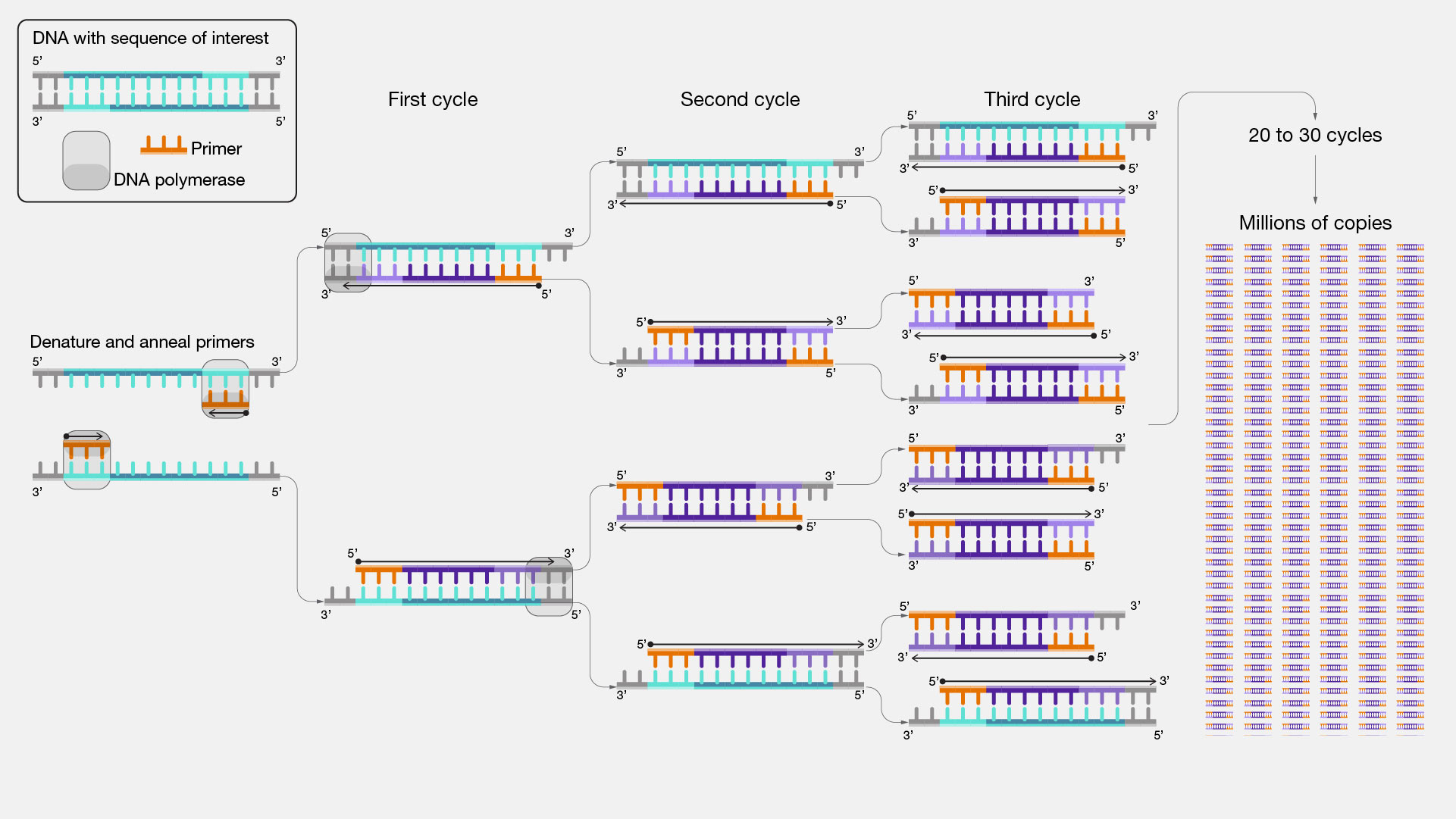
Fig. 2.19 The polymerase chain reaction uses primers to select a desired region of DNA, and doubles it’s reaction products every cycle. Credits: [National Human Genome Research Institute (NHGRI), 2024].#
PCR primers typically have to meet several requirements to result in a successful PCR product: they have to be biochemically feasible (i.e. denature, anneal, and extend at the right temperature), they have to be specific (only amplify the region of interest), they should produce a product of a reasonable size (~500-1000 nucleotides, depending on the application), and they should be stable as single stranded DNA. The combination of these requirements typically allows primers of ~18-30 nucleotides long. To aid in the quick design of potentially successful primers, tools such as Primer-BLAST or Primer3+ automatically check most of the mentioned requirements. For example, Primer-BLAST lets a user upload a sequence of DNA that should be amplified, and can be configured to find primer products of a specific size. In addition, putative off-target amplification (i.e. specificity) is checked using BLAST on a database of choice, and several desired temperatures can be configured.
Approximating PCR denaturation temperature \(T_m\)
The temperature at which approximately half of the DNA strands in a solution are in a denatured stated is referred to as the melting temperature \(T_m\), and is an important parameter in primer design. The exact melting temperature depends on the exact length and nucleotide composition of the DNA fragment, but for short sequences a useful approximation exists. This approximation can come in handy for quick checks and predictions.
For primers shorter than 14 nucleotides, the melting temperature can be approximated with the following formula:
\(T_m = 2 * (A + T) + 4 * (G + C)\)
Where A, C, G, and T are the number of respective nucleotides in the primer.
Practical assignments#
This practical contains questions and exercises to help you process the study materials of chapter 2. There are two supervised practical sessions, one on Wednesday and one on Thursday. On the first practical day you should aim to get about halfway through this guide. Thus, you should aim to be finished with Assignment III. Use the time indication to make sure that you do not get stuck in one assignment. These practical exercises offer you the best preparation for the project. Make sure that you develop your practical skills now, in order to apply them during the project.
Note, the answers will be published after the practical!
Assignment I: Protein sequence BLAST of Vps36 (30 minutes)
Finding homologs of proteins is a common task in biology, since the presence of homologs can tell us something about the function of the protein and in which other species it can be found.
Thus, we first practise finding homologs.
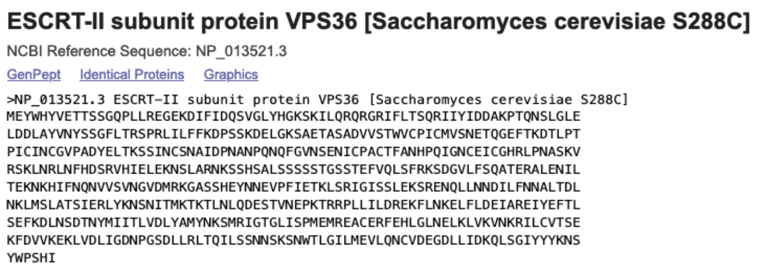
We want to find homologs of the yeast protein Vps36, the Vacuolar protein-sorting-associated protein 36.
To this end, we search in two different databases and compare the results.
Retrieve the protein sequence of Vps36p from the yeast S. cerevisiae (NP_013521.3) from NCBI in fasta format. (Note: you can download it into a file or leave the tab open and use copy/paste). What does the fasta format look like? I.e. how is the sequence and the additional information (name) of the sequence stored?
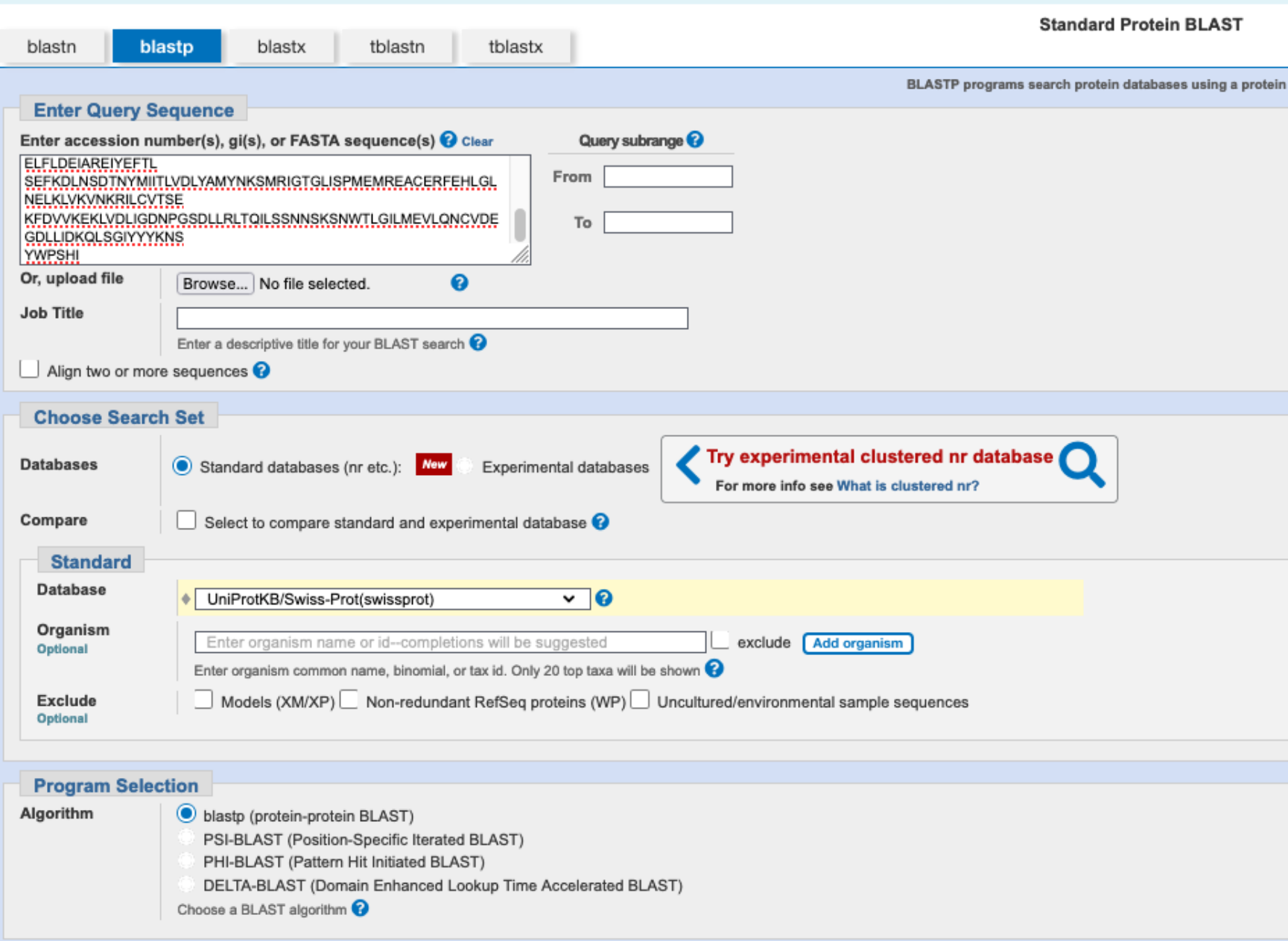
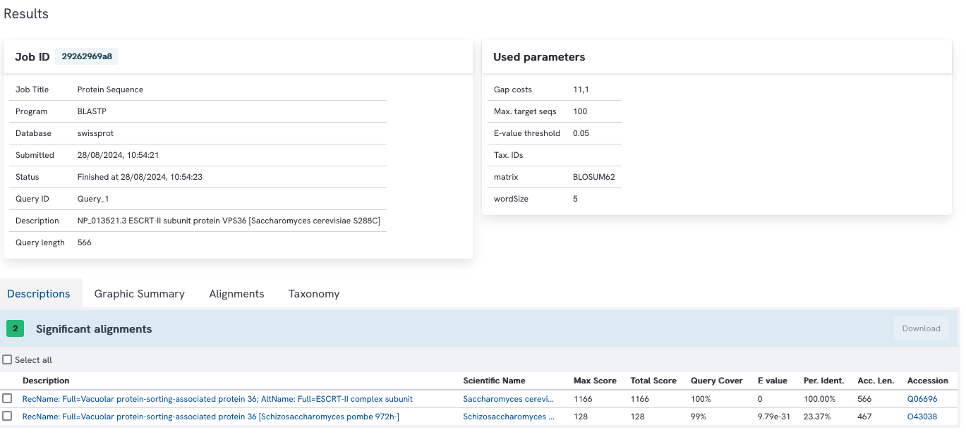
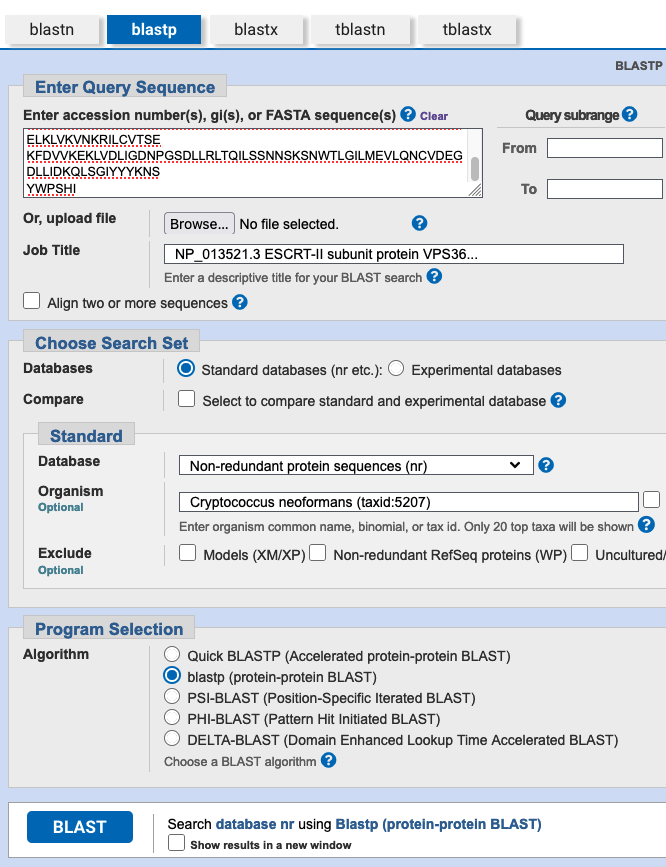
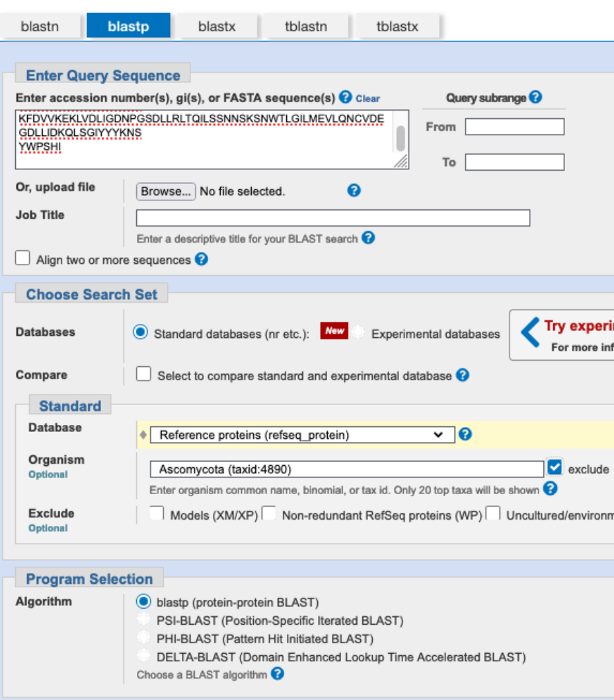
We want to identify similar proteins in the swissprot database using the National Center for Biotechnology Information (NCBI) BLAST program. Go to the website of the NCBI. On the right side of the webpage, you find a direct link to BLAST. Next, you need to decide which search strategy would be appropriate to search a protein database (swissprot) with a protein sequence as a query (if you are not sure anymore, look at Fig. 2.15). Click on the appropriate search strategy. Enter the sequence into the query box, select UniProtKb/Swissprot as the database you want to search, and make sure you have the correct algorithm selected. Finally, click on the ‘BLAST’ button to perform the search.
Have a look at the result page of your search. Where can you find information about your query, an overview of the database hits obtained, the distribution of these hits on along your query sequences, and the alignments between the query and each individual database sequence?
In which organisms do you find similar sequences? Which of the hits do you consider as homologs?
What is the interpretation of an e-value? What does an e-value of 0.0 suggest?
The NCBI blast service is an important bioinformatics tool, that you should practice. However, we have experienced that high usage from one location at the same time (like during BIF20306 practicals) results in a delayed response of the web service. To mitigate long waiting times, we set up a server with the most important NCBI blast functionalities. Run the previous search also with this server and look at the results. Note that with the run url you will also be able to retrieve the results later. Preferably, do all the following blast exercises in Assignments I and II with this server.
Next, we want to find more homologous sequences; thus we search in the RefSeq protein database (Blast database refseq_protein). How many hits do you find? Look at the last hit, do you think that all similar sequences in that database have been found? Note: We still need the results in Swissprot. Save the urls, so you can retrieve them later or leave these results open and perform the new search in a new browser window or tab.
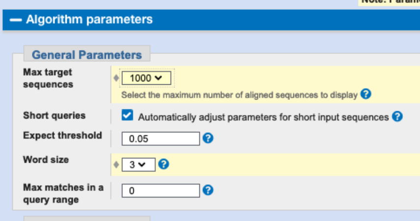
Perform the same search as in (7), but now allow for finding a larger number of hits (Change Max target sequences under Algorithm parameters to the maximum available). How many hits do you find? Would you consider all of them as homologous to the yeast Vps36?
Go back to the Swissprot results and look at the first hit that is not the query sequence itself. Compare the blast results (score, query coverage, e-value, percent identity, alignment length) to the hit of the same species found in RefSeq. What do you observe?
Assignment I answers
Fasta label always starts with a
>. The protein/nucleotide sequence follows in the coming lines; see also Blast documentation.
The information is displayed in the browser, under different tabs (Descriptions, Graphic Summary, Alignments, and Taxonomy).
Two hits are found in two different yeast species. They both have low e-values and match over the whole length, but one has also low identity.
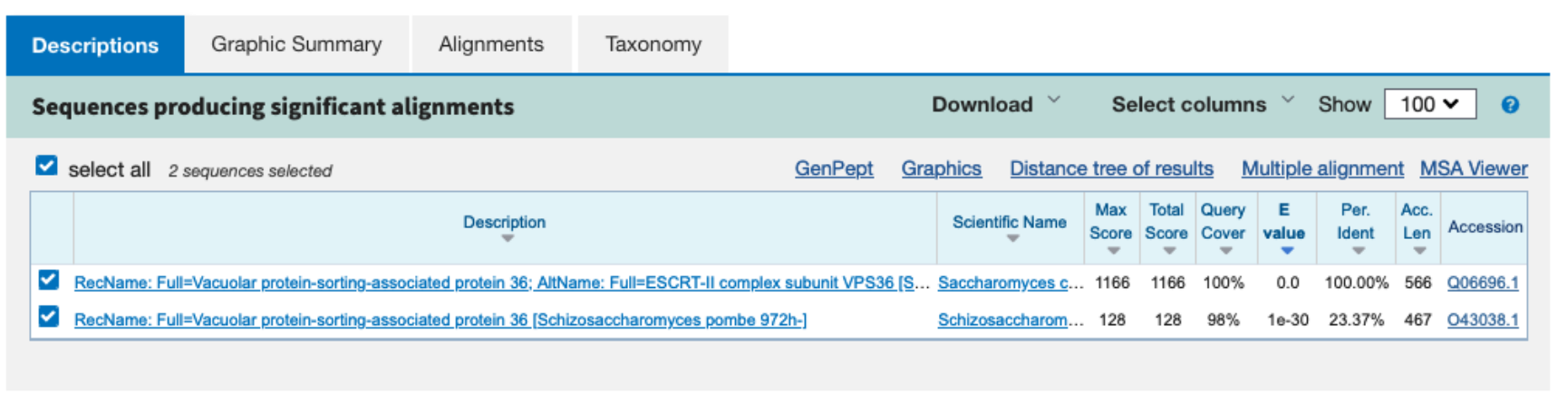
The E-value represents the number of alignments with a score of at least S that would be expected by chance alone in searching a complete database of n sequences. The E-value is used to order the BLAST results. A low E-value indicates that a hit is significant. An E-value of 0.0 means 0 sequences are expected to match with this score (or higher), so this indicates a highly significant hit.
We perform another search in swissprot.

We find two hits again.
100 hits are found, the last one has an e-value of 6e-42 (with NCBI blast) or 2e-42 (with WUR blast), thus the list is probably incomplete and only the first 100 sequences are reported.
With WUR blast 591 hits are found (with NCBI blast, 587 hits would be found, probably due to a slightly different database version). Most hits have low e-values, but some have high e-values (above 0.001) and might not be considered homologs.
All the results are the same, only the e-value is lower with the Swiss-Prot database. Thus, the found proteins are identical, but the refseq database is much larger, which results in a higher e-value.
WUR blast result with RefSeq database

NCBI blast result with RefSeq database

Assignment II: Some more BLAST, with flavors (60 minutes)
Blast cannot only be used to search protein sequences in protein databases with blastp, but also offers different blast flavors that either allow to search in databases of different type (see Fig. 2.15) or with alternative search strategies and also to restrict the search to particular species. Here we explore these strategies by searching for homologs of the yeast Vps36p in fungi and other organisms.
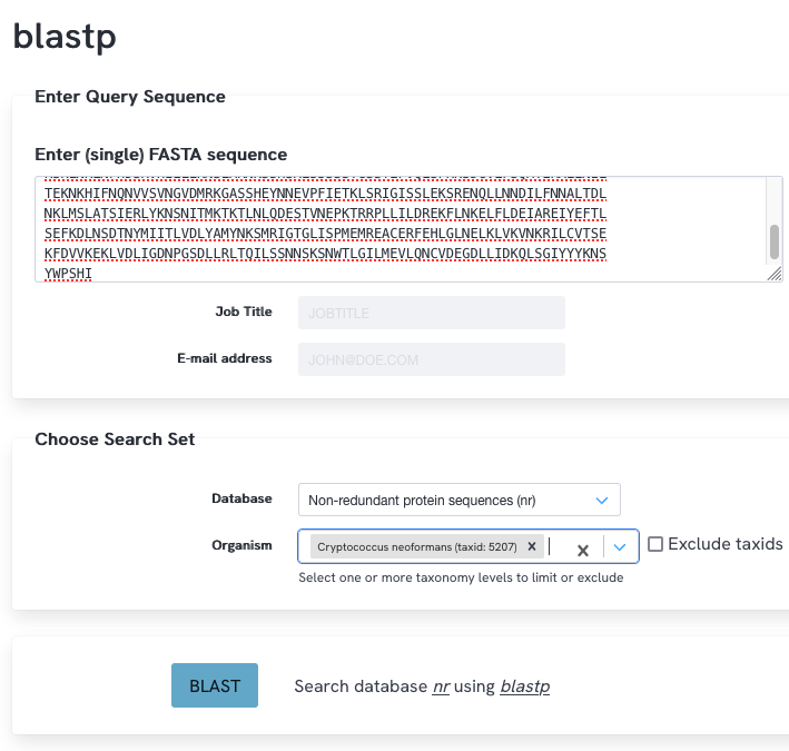
Next, we aim to find out if homologs of this protein exist in the fungus Cryptococcus neoformans. What would be the most straightforward BLAST search strategy to do this? Perform this blast search using a large database (Non-redundant protein sequences (nr)). How many hits do you find? Inspect the length of the alignments, the percent identity, and E-value. What do you observe and what do you conclude?
In case no homologs would have been found using a ‘normal’ blastp search, which alternatives could you use to still find homologs, e.g., in the genome sequence? Describe what happens in that BLAST flavor.
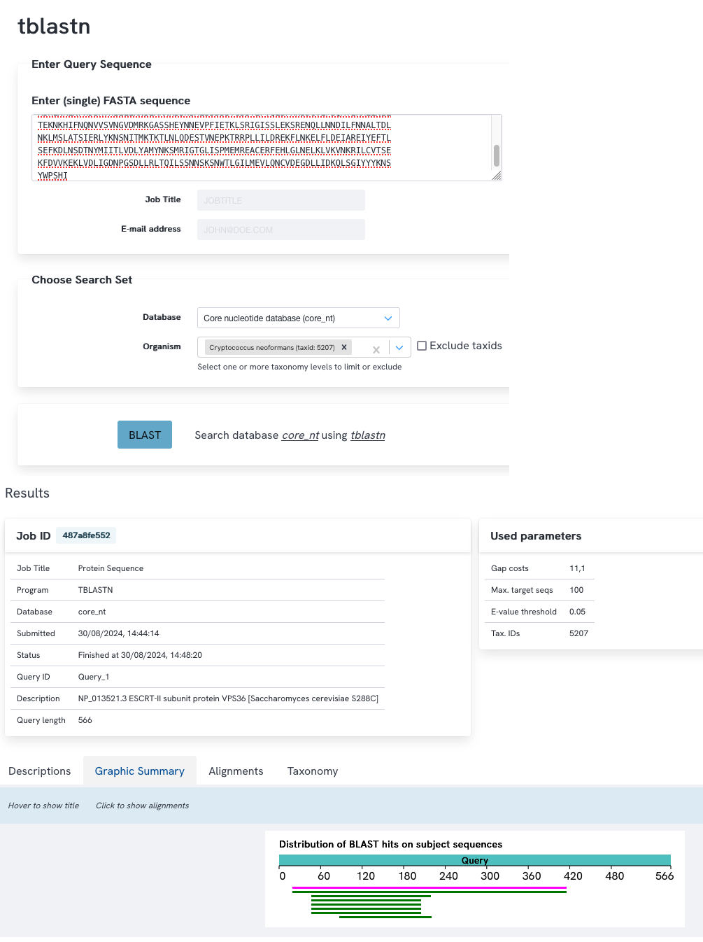
Search the protein sequence of Vps36p against the nucleotide sequences of C. neoformans using tblastn, indicating that you only want to search this single species and not the entire database (use the database: Core nucleotide database (core_nt)). Inspect the search results. Do you think these are good hits and would you feel comfortable to conclude that there are (or are not) homologs of this gene in C. neoformans?
Some of the hits reported are part of chromosome 1 of C. neoformans. Inspect these hits in more detail. How long is your query and how long is the sequence in the database?
Think about the following case, where you would like to study this hit in more detail. For instance, you could perform a multiple sequence alignment of your protein with this database hit and also with other sequences. What would happen if you would download the sequence from the database? Why could this be a problem, and how could you solve this?
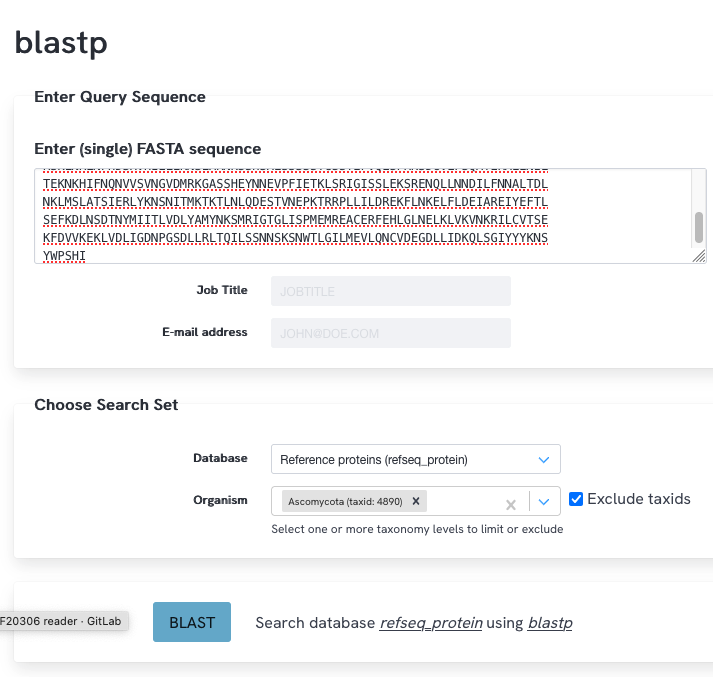
S. cerevisiae belongs to the fungal phylum Ascomycota, while C. neoformans belongs to the phylum Basidiomycota. Vps36p is highly conserved throughout Ascomycota and likely has homologs outside of this phylum too, as already indicated by your searches above. We now want to get a better overview of possible homologs of Vps36p in other species (outside of Ascomycota). To this end, perform a blastp search of Vsp36p to the refseq_protein database (excluding Ascomycota), set the number of target sequences to the maximum. Have a look at the best hits. What can you say in terms of query coverage and identity?
Take a look at the taxonomy report of your results (link on top of the blast result page). In which groups of species did you find hits?
At least one of your hits is outside of fungi, suggesting that Vps36p homologs might be more widespread. What could be a possible blast strategy to find more distant homologs?
Try to modify the Algorithm parameters for the search done in (6). To find more homologs, keep using the blastp algorithm, just try to modify a parameter. How many hits do you find? Finally, we want to get an overview how similar these distantly related proteins are. To this end, we will download some hits and perform a multiple sequence alignment.
Generate a multi-fasta file of 10 sequences: The first 9 hits from the previous blast search and the original sequence (NP_013521.1). (Hint: you can mark sequences and save them by clicking on Download -> Fasta (complete sequences); use a text editor to add the original sequence manually).
We will use M-Coffee from the T-Coffee suite. This program uses multiple other tools to compute several multiple sequence alignments and combines them into one final alignment. The output includes a color code showing the agreement between the methods. Upload you multi-fasta file and run it with default parameters. Look at the estimated alignment. What can you say about the overall alignment quality? Where can you find regions of high and low agreement?
Would you conclude that these sequences are homologous across their entire length? Why/why not?
Assignment II answers
WUR blast
NCBI blast
A regular blastp against the proteins of Cryptococcus neoformans could be done (database nr, limit search to Cryptococcus neoformans (taxid:5207)). You find 21 hits. Several hits have a good query coverage (>75%) and low E-value, but all these hits have a low percent identity (around 22%), suggesting these might be very distant homologs. The hits at the bottom of the list cover only a very small part of the query, and have a high e-value, so these are irrelevant.
Try to find matches to DNA, for instance by using TBLASTN (Protein query searching six-frame translated DNA database). BLAST parameters could be adjusted, e.g., the word size could be decreased to include more distant sequences. PSI-BLAST will not work as it only will be able to find more distant matches once the first iteration yields results.
WUR blast
NCBI blast
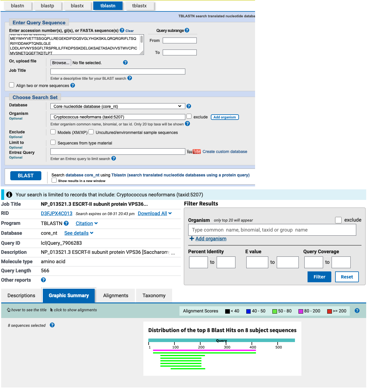
You find 8 hits. The results are similar to the blastp results. The first two matches have a good combination of a low E-value and a high query coverage. However the percent identity is low. This suggests these are clearly divergent (low percent identity) homologs in C. neoformans. The other hits concern only a small part of the query.
WUR blast

NCBI blast
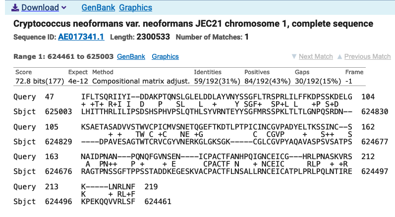
The query is a protein and thus short (566); blast is performing a local alignment and the complete sequence database match is in this case very long (part of chromosome 1), around 2.3 Mb.
You will likely get issues with the alignment, even with a local alignment. The aim of an alignment is always to align homologous sequences, but if you offer an entire chromosome, the alignment tool will nevertheless align the sequence, which likely will not yield meaningful results. An option would be to slice the sequences around the match (i.e., cut out the matching part) from the database sequence and use this data for the alignment.
WUR blast
NCBI blast
There are 116 hits (with NCBI blast that would be 118). The top hits are good (low e-value) with good query coverage within the other species outside of Ascomycota. The percent identity is relatively low ~25% in these hits, because of the evolutionary distance between S. cerevisiae and species outside the phylum Ascomycota.
The hits are mainly fungi, but also few non-fungal matches, suggesting this protein may be more common in other species as well.
To identify related sequences that are too dissimilar to be found in a straightforward BLAST search, the word size could be decreased or PSI-BLAST could be used.
We can modify the word size, this is expected to yield more distant hits.
WUR blast
NCBI blast
We then find 190 hits (with NCBI blast, that would be 193).
All 10 sequences, each starting with their Fasta label, should be copy/pasted into one Fasta file.
The alignment looks good. The beginning is very well aligned with few gaps. Although there are stretches containing gaps, there are also long regions throughout the alignment with no or few gaps and these are of good quality. Nevertheless, there are also low-quality regions.
From the observations in the previous question, you can conclude that these are homologous sequences over their whole length.
Assignment III: Analyses of the PLT1 family - part 1 (60 minutes)
Stem cells are undifferentiated cells that can differentiate into specialized cells and therefore are crucial during embryonic development of different tissues and for growth. In plants, such as the thale cress Arabidopsis thaliana, stem cells are found in specific regions in the roots and shoots, thereby providing a continuous supply of specialized cells required for these tissues. PLT1 is a transcription factor that is required to maintain stem cells in the root (Aida et al. 2004). Here, we will use bioinformatics approaches to analyse PLT1 to discover if it is part of a larger gene family and which related sequences exist in A. thaliana.
UniProt is a publicly available protein database that contains protein sequences and functional annotation for >200,000,000 protein entries.
Have a look at the UniProt website. Why does UniProtKB-TrEMBL have so many more entries than UniProtKB-Swiss-Prot?
Search for the Arabidopsis protein PLT1 using the UniProt identifier Q5YGP8. The PLT1 entry provides you with an overview of the protein entry and some functional information. Read the functional description of PLT1. Does this description fit the information above on PLT1, and how does UniProt gather this information?
Which functional regions are present in PLT1? Where in the sequence are they located? Which database is used for that information? (Hint: functional regions can be found under Function -> Features).
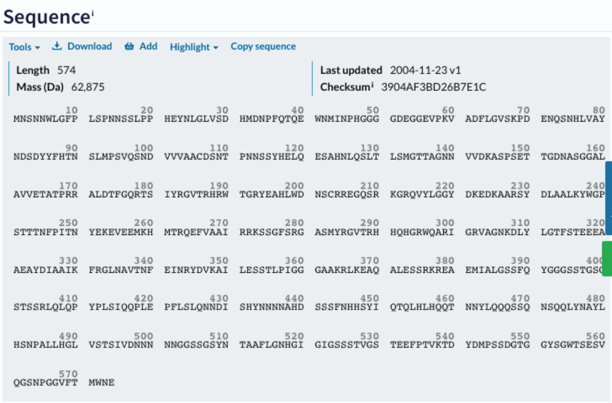
Towards the end of the entry, you can find the actual protein sequence of PLT1. You can download the sequence in fasta format by clicking on the Download button.
Interpro also provides a functional analysis of proteins and their domains. Go to the interpro website and look up the entry for PLT1. How many protein domains have been identified in PLT1 and where are they located?
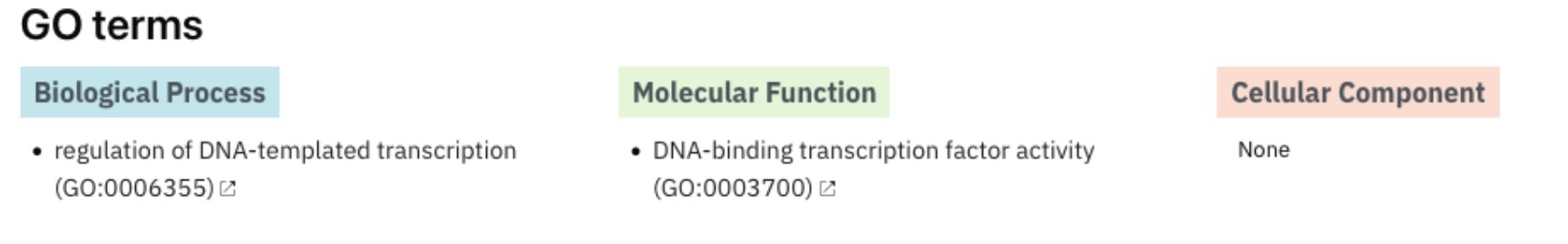
Look up the domain in Interpro. What is the function of the identified domains? What information can you find on GO terms and on protein structures?
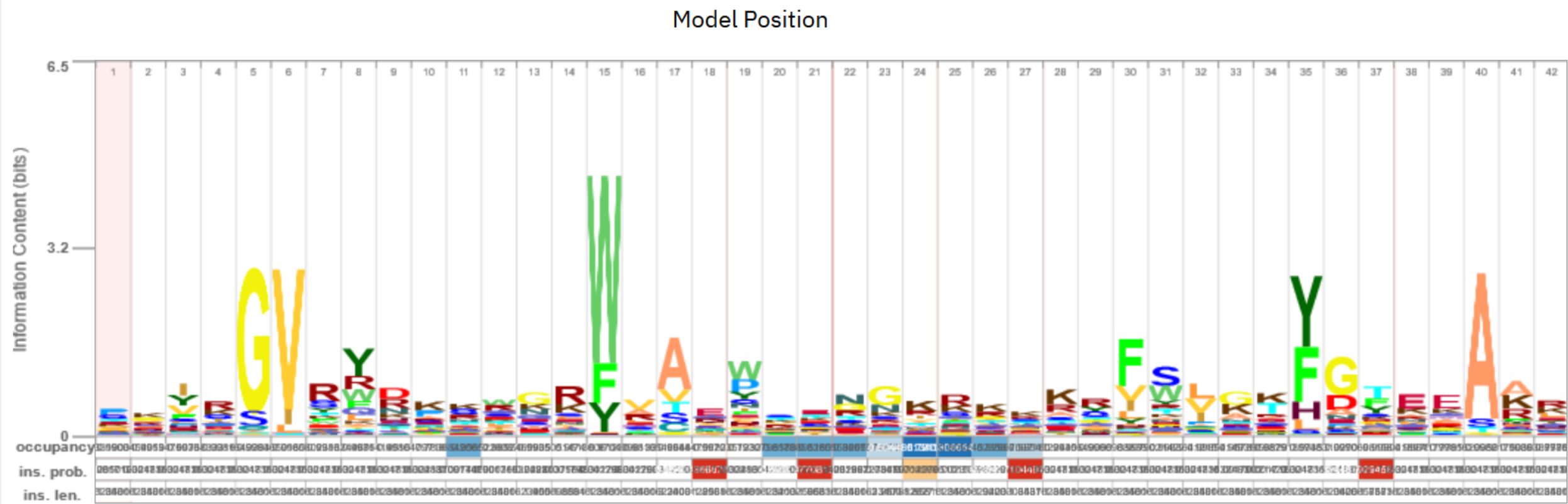
Look up the domain in Pfam and look at the HMM logo of the domain. Which 3 positions are most conserved and which amino acids are preferred there?
We want to analyze the repeats in this protein using the online dot-plot program Dotlet. Go to the website and add the PLT1 protein sequence as sequence 1 and sequence 2 (we want to perform a self-comparison). To filter some of the low scoring alignments you need to use the sliders below the score histogram. How many repeats can you find in this segment of the protein, and at which locations within the protein fragment are these located?
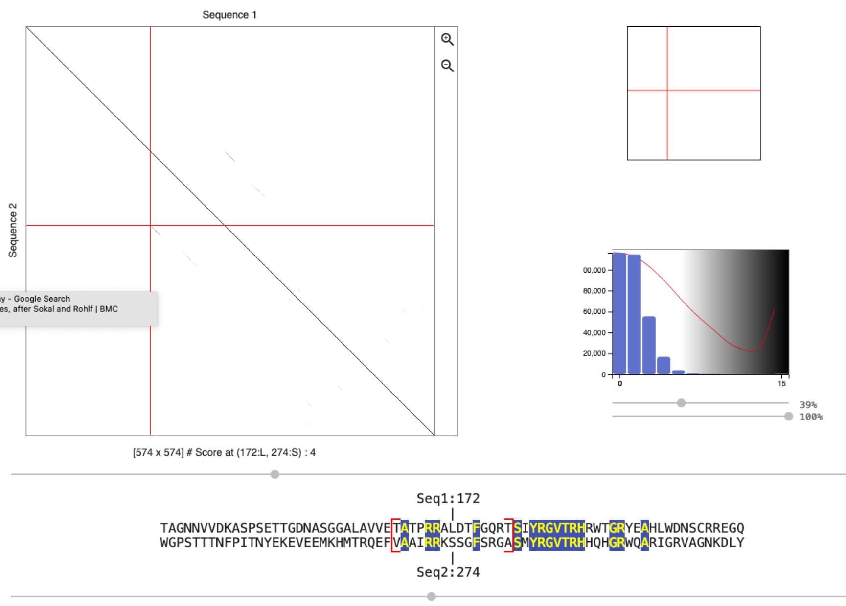
What happens if you change the scoring matrix from
BLOSUM62toIdentity?Use the mouse to click on the region that likely contains the repeat sequence. Use the left and right arrow keys to locate the beginning of the aligned repeat structure. Which conserved amino acids can you identify? Compare the logo of the repeat family with the conserved amino acids that you found. What do you observe?
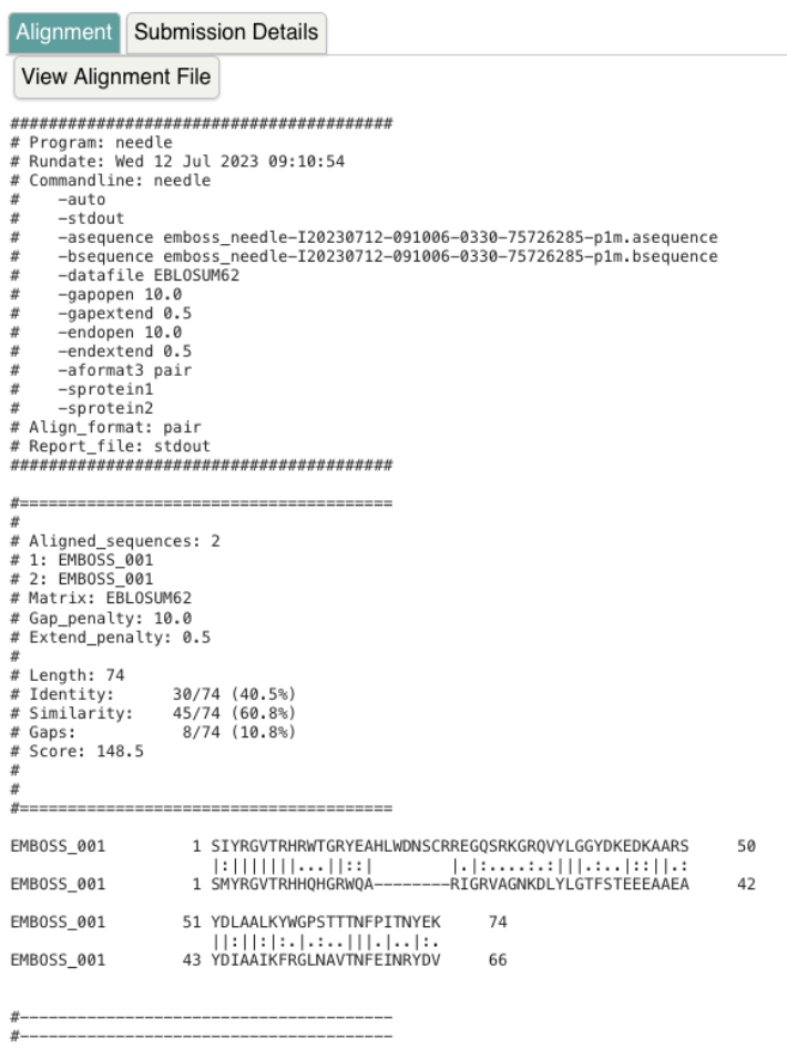
Pairwise sequence alignments can identify regions that are conserved. Obtain the amino acid sequence of the first and second AP2 domain of PLT1 that was found in InterPro and perform a pairwise sequence alignment with algorithms you can find on the EBI website. First perform a global alignment using the Needleman-Wunsch algorithm (Needle). Choose protein alignment and add the protein sequence of each of the protein domain sequences of PLT1. What is the overall identity and similarity between the two domains, and why do these two values differ?
Now perform a local alignment using the Smith-Waterman algorithm. Do you expect to observe large differences between the global and the local alignment? Explain why.
Assignment III answers
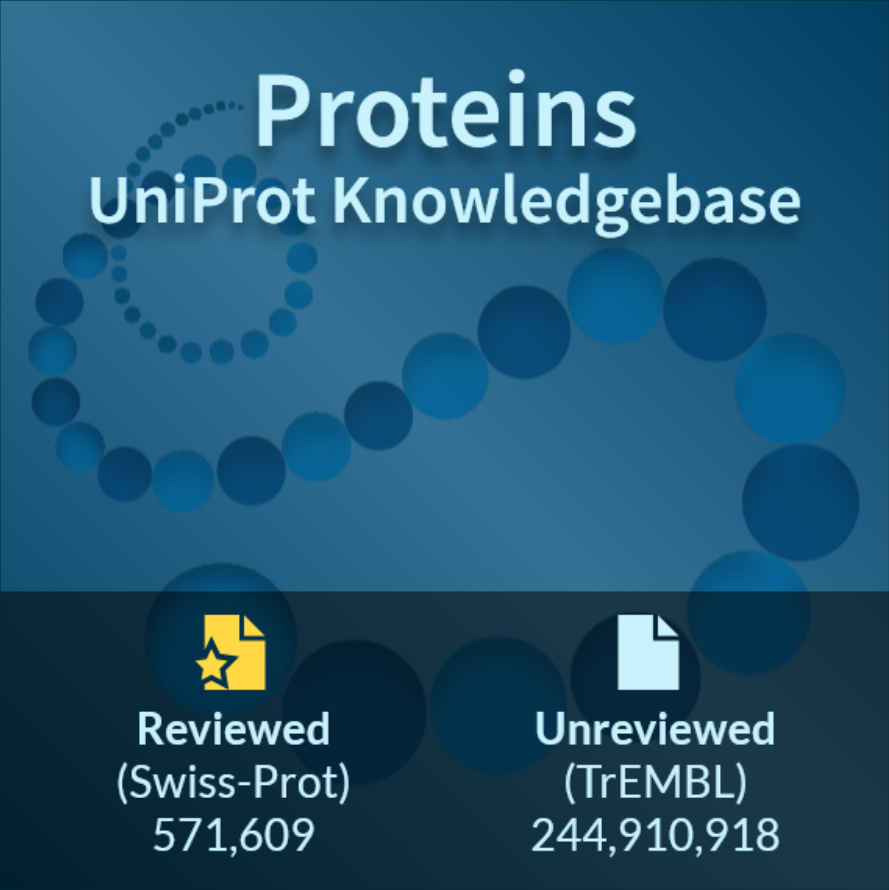
Swiss-Prot contains manually annotated sequences while TrEMBL contains automatically deposited sequences (for instance from genome sequencing projects); UniProtKB contains data from both databases.
PLT1 is a transcription factor. This is mainly based on sequence similarity but also based on information from literature.
UniProt reports two AP2 domains. According to Prosite, they are located at positions 181-247 and 283-341 in the protein.
Use the browse function and enter the Uniprot accession. You can identify two AP2 DOMAINS (IPR001471/PF00847). IPR001471: 180-253 and 282-347.
AP2/ERF domains are transcription factors. 8 structures are found in PDB, 49K structures are found in Alphafold.
15(W), 6(V), 5(G).
There are 2 repeats, starting around 170 and 270.
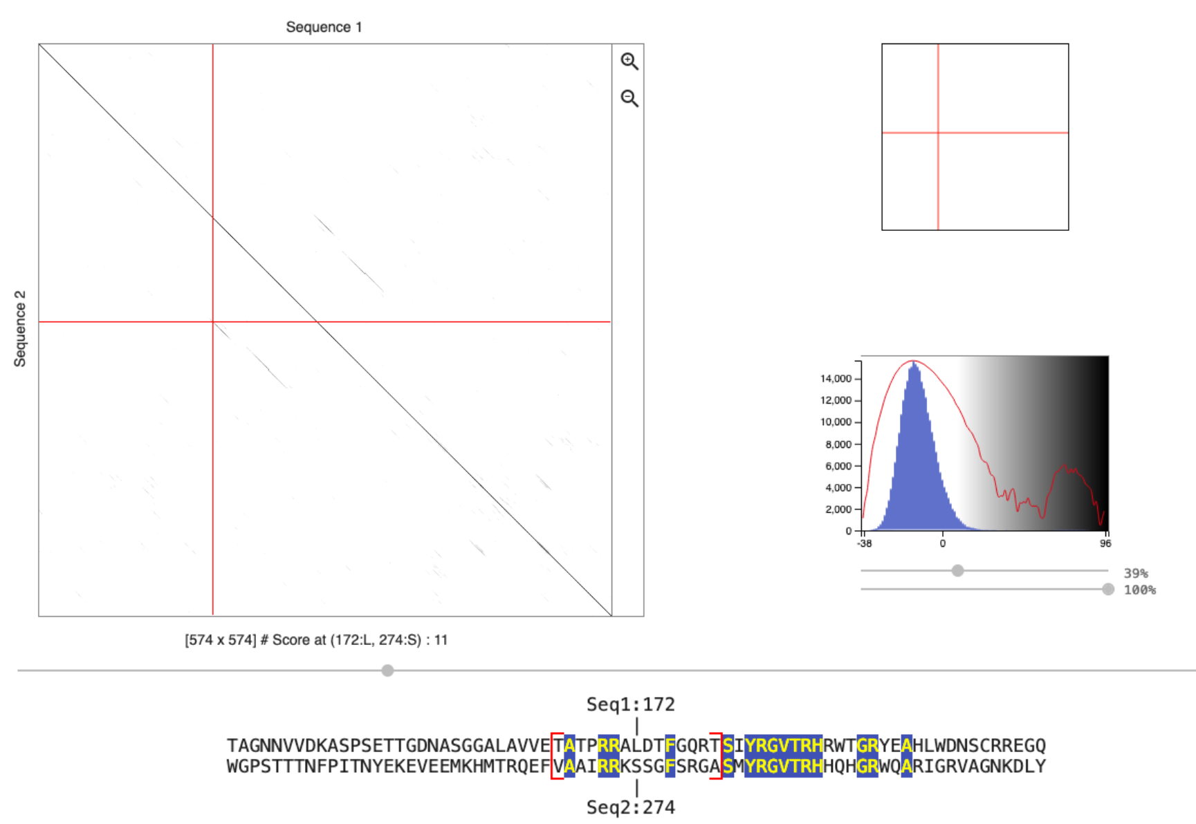
Identity only scores sequence matches (typically +1) and thus the score distribution only has values ranging to the window size (the cutoff, used to determine if a dot is plotted in the dotplot, can be changed using the slider). The BLOSUM scoring matrix also gives a score to mismatches and thus the range of possible scores per window is bigger (see distribution). The same repeats are identified, but they are easier to see with the BLOSUM matrix.
Some of the conserved amino acids can be identified (GV).
You can obtain the sequences by clicking on the range after hovering over the accessions in question g. The range is then marked and can be copied (you may have to get rid of the gaps). Another option is to obtain the domain sequences from UniProt -> Function -> Features -> Sequence.
Note that the positions differ slightly. With the Uniprot regions, the alignment length is 67 (identity 40.3%, similarity 61.2%). With the Interpro regions, the alignment length is 74 (identity 40.5%, similarity 60.8%, see screenshot). Using the identity score only identical residues are counted; using similarity, also amino acids with similar properties are counted.
One would not expect too many differences as the alignment already only concerns domains and not the entire protein sequence.
Assignment IV: Analyses of the PLT1 family - part 2, finding homologs (30 minutes)
After we analysed the PLT1 sequence, we want to find potential homologs of PLT1 in the thale cress Arabidopsis thaliana. We will use BLAST to identify protein sequences in publicly available databases with sufficiently high similarity scores such that these are likely homologs of PLT1.
Go back to the UniProt database and click on BLAST within the UniProt entry. Change the target database to “UniProtKB Swiss-Prot” and perform the search (‘Run BLAST’). What is the ‘best’ hit found (how could you define ‘best’)? Look at the second-best hit, which sequence is that and in which organism is it found? Report the e-value, the identity, and the score. How might the two sequences be related?
How many hits do you find with that search?
Do you expect to find even more database hits in the UniProtKB database than what your original search showed? Why? Which of the included database would be the most useful database to identify PLT1 homologs in plants? Why?
How could you influence the number of hits you find in the database?
Repeat the search, but only consider hits with an E-value of 1e-4 and up to 1,000 possible matches. How many hits do you find?
Now we want to focus on homologs in A. thaliana (click on A. thaliana in popular organism). How many hits do you find in A. thaliana?
On the right part of the output page, you can find a graphical overview of the alignment (aligned part highlighted as thick bar). You can also click on these to see the aligned regions. If you look at the first ten sequences, what do you observe regarding the aligned region, and what does this suggest? Is this what you would expect from a BLAST search, and why?
Save the first ten database hits in fasta format. Note: UniProt provides an alignment option, which provides the easiest way to get all sequences of interest: Mark them -> click Align -> click Align selected results -> copy the sequences from the window into a text file, take care to copy the whole 10 sequences.
Assignment IV answers
The first hit is the query itself (ID Q5YGP8), 100% identity. The 2nd match has lower identity (74%), but also an E-value of 0.0, score 2122, covers the whole query. The hit is PLT2 also found in A. thaliana. The 2 sequences might be related by a duplication.
250 hits. The limit on the number of returned alignments was set to 250.
You would likely find more than 250 hits; 250 is set as default, always check the default settings of the programs you use. Swiss-Prot hits are likely better than TrEMBL due to the increased quality (manual vs automatic).
Set the E-value parameters and/or the max number of matches. On the results page you may also select ‘popular organisms’ to only get results from these.
136 hits are found.
104 hits.
BLAST always performs a local alignment. Most of these hits only cover parts of the target sequence, which is expected for a local alignment. The more sequences diverge, the smaller the identity and the region with sufficient similarity to perform the alignment will get. This is normally also reflected by drops in bit-score and e-value. Thus, when filtering matches on identity, query coverage should also be considered.
Make sure you save the first 10 database hits in fasta format somewhere you can find it again. You will need it for the next assignment.
Assignment V: Analyses of the PLT1 family - part 3, conservation (30 minutes)
Next, we want to explore the conservation of the PLT1 family identified in the previous assignment. To this end, we use multiple sequence alignments.
Use the first ten hits from the Swiss-Prot database (see assignment IV, question 8.) to perform the multiple sequence alignment using MAFFT. Download this alignment in FASTA format and save it somewhere you will be able to find it again. You will re-use this alignment in Chapter 3 to build a phylogenetic tree.
Which regions are well aligned, and which not? How can you easily spot these in a multiple-sequence alignment? How does this region relate to the previously identified protein domains?
Look at the iterative refinement methods available as options in MAFFT. Which strategy do you find appropriate for your data set?
Run the strategy that you propose and compare it to the previous alignment. What do you observe? Check the results page of the first run again. Can you find an explanation for your observation?
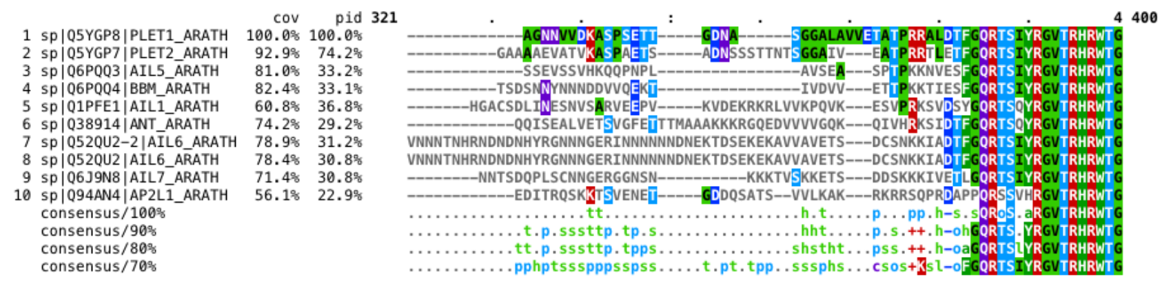
Download the first multiple alignment (question 1) in fasta format and display it in an alignment viewing program. Locate the start of the first AP2 domain in the alignment (Hint: look at the Pfam logo and try to find the first 2 highly conserved positions). Where does the domain start? Look at the first 10 positions of the domain and compare the conservation in the alignment to the Pfam logo. What do you observe?
Next, we try a different alignment tool: M-Coffee from the T-Coffee suite. Does that tool provide a good global alignment? Why/why not?
The T-Coffee suite also includes a program to extract reliable regions from an alignment: the Core/TCS tool. We want to use this tool to extract reliable columns from our alignment. Use the button under “Send results” -> Core/TCS at the bottom to run it, then click “Submit”. A fasta file, where only the well aligned columns are included, can be downloaded at the bottom (“fasta_aln file”). Display this file in mview. What can you say about the quality of this alignment?
Assignment V answers
Make sure to save the alignment in FASTA format somewhere you can find it again. You will need it for the practical assignments of chapter 3.
The two AP2 domains are well conserved, while the N and C terminus are generally less well conserved. The conserved columns are marked with a
*. We find that only the domains are well aligned in the global multiple alignment, which is in accordance with the earlier observation that we only found local hits (assignment IV, question 7).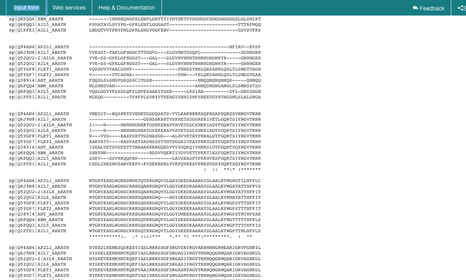
We saw in blast that they only partially overlapped with the query in a region containing the AP2 domains. Thus, E-INS-i or L-INS-i would be appropriate.
The results are very similar (or identical). The auto option had already choosen the appropriate L-INS-i strategy.
Try to locate the conserved GV and then go 4 positions back. The resulting position is 389, it contains a conserved S. The first 10 positions are conserved in the alignment at 70% consensus: SIYRGVTRHR. They are less conserved in the AP2 domain logo since that is based on more sequences from different organisms.
This tool is also only aligning some regions well. Only parts of the proteins might be homologous.
This alignment is much shorter, it only includes well aligned columns.
Assignment VI: Discovering protein families (20 minutes)
Next, we are interested in another yeast protein – PMP2 (A6ZQT2) – and its homologs.
Look up PMP2 in UniProt and blast it against UniProtKB with an e-value threshold of 0.01. How many hits do you find?
Next we try to find distant homologs using the HMM-based tool jackhmmer. Read the first paragraph here to learn about this tool. Why are more hits found in subsequent iterations?
Go to jackhmmer and search PMP2 in the database UniProtKB. How many hits do you find in the first iteration?
Start the second iteration with the button on top. How many hits do you get now?
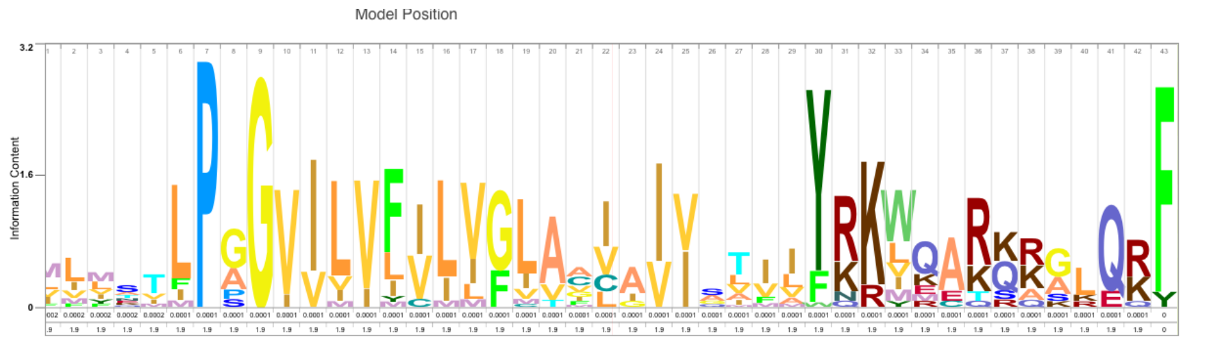
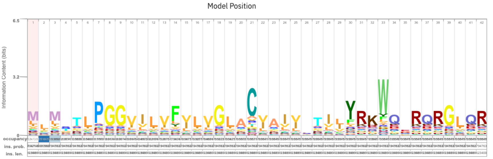
Look at the model in the bottom of the results page. What do you see here? What can you say about the conservation of particular amino acids?
Now we want to check if it is known already that this protein belongs to a larger protein family. How could you find this out?
Look up if there is a Pfam domain known for this protein. What is known about its function according to the Pfam domain?
On the website of the Pfam domain, you can find the corresponding logo under “Signature”. Compare the logo of the family to the logo found with jackhmmer. What do you observe?
Assignment VI answers
55 hits, 54 are in fungi, 1 in a Sar eukaryote.
It builds an HMM from the hits which is then used to find more distant homologs.
54 hits.
236 extra hits, 290 hits in total.
There is the logo of an HMM model, positions 7(P), 9(G), 30(Y), and 43(F) are particularly conserved.
We could check UniProt or InterPro with the UniProt accession A6ZQT2.
We can look up the UniProt accession in InterPro. We find PF08114: This family consists of small proteolipids associated with the plasma membrane H+ ATPase.
We find some congruent positions, e.g., starting at 5: TLPGGVILVF. But there are also differences, e.g, Pfam shows C in pos. 21.
Assignment VII: Motif discovery in bacteria (20 minutes)
The bacterial immune system CRISPR/Cas encodes the defense sequences to target mobile genetic elements in the CRISPR (clustered regularly interspaced short palindromic repeats) locus, where the defense sequences are located between repeats. Here we will use motif discovery to determine the repeat sequences.
Access the RefSeq database at NCBI to retrieve the genome data for Streptococcus thermophilus (Accession NZ_LR822015.1). Hint: Use Customize view to display all features
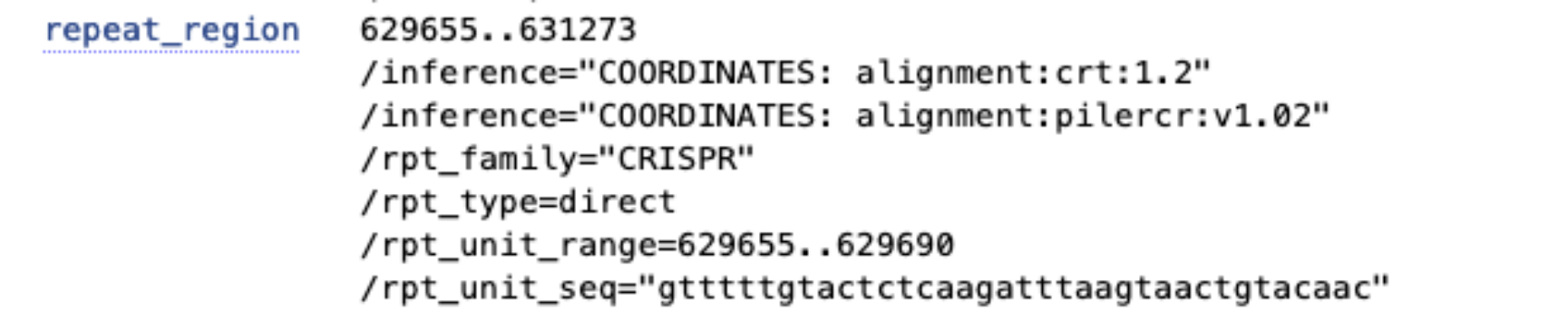
Go the the first
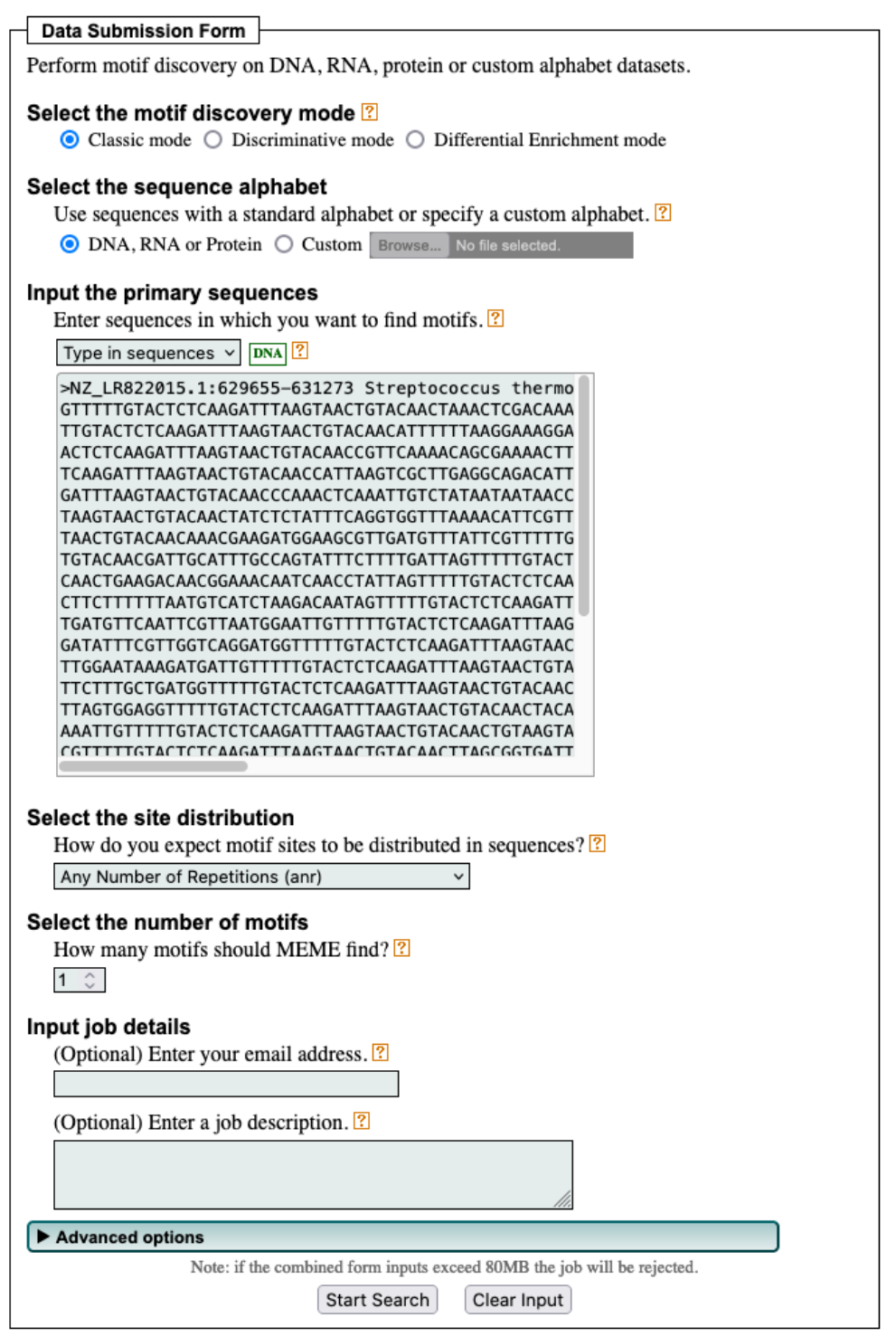
repeat_regionfeature. Where in the genome is it located? Retrieve the sequence of this feature (Hint: click onrepeat_regionand then onFastain the bottom right).Use MEME and MAST to discover the motif. Go to the MEME suite and click on MEME. Under Input, select “Type in sequences” from the dropdown menu to paste your fasta sequence. Choose the correct option under “How do you expect motif sites to be distributed in sequences?” and select one motif to find.
After running the search, retrieve the MAST HTML output. Which motif do you find and how often does it occur in the sequence? Compare the motif to the repeat annotated in RefSeq. What do you observe?
Assignment VII answers
You can access the RefSeq database from the NCBI website.
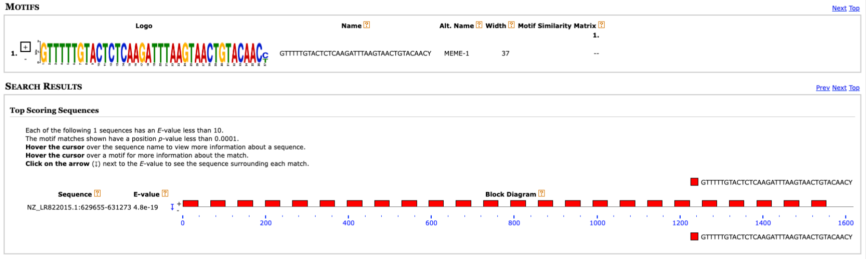
The found motif is very similar to the repeat region (
gtttttgtactctcaagatttaagtaactgtacaac). The motif is even one base longer indicating that C and T are preferred at the first nucleotide of the defense sequence. MAST finds it 24 times.
Assignment VIII: Primer design for the Phytophthora infestans effector gene Avr1 (30 minutes)
Phytophthora infestans is the causal agent of tomato and potato late blight disease. Potato late blight had significant historic impact in Europe and North America as it led to the Great Famine in Ireland in the middle of the 19th century, where one million inhabitants of Ireland died and another million emigrated to the United States of America. P. infestans, as many other plant pathogens, utilizes so-called effector proteins to establish themselves in susceptible plant hosts. The Avr1 gene in P. infestans encodes an effector Avr1 that contributes to virulence in susceptible potato plants, yet is recognized by the plant immune system in some resistant potato varieties. Therefore, to avoid recognition by the plant immune system, some P. infestans isolates lost the Avr1 gene. Recently, a farmer collected different P. infestans isolates from his fields around Wageningen, and the farmer wants to know if these isolates contain Avr1. Here, we aim to design primers that can be used to detect the presence of the Avr1 gene in P. infestans.
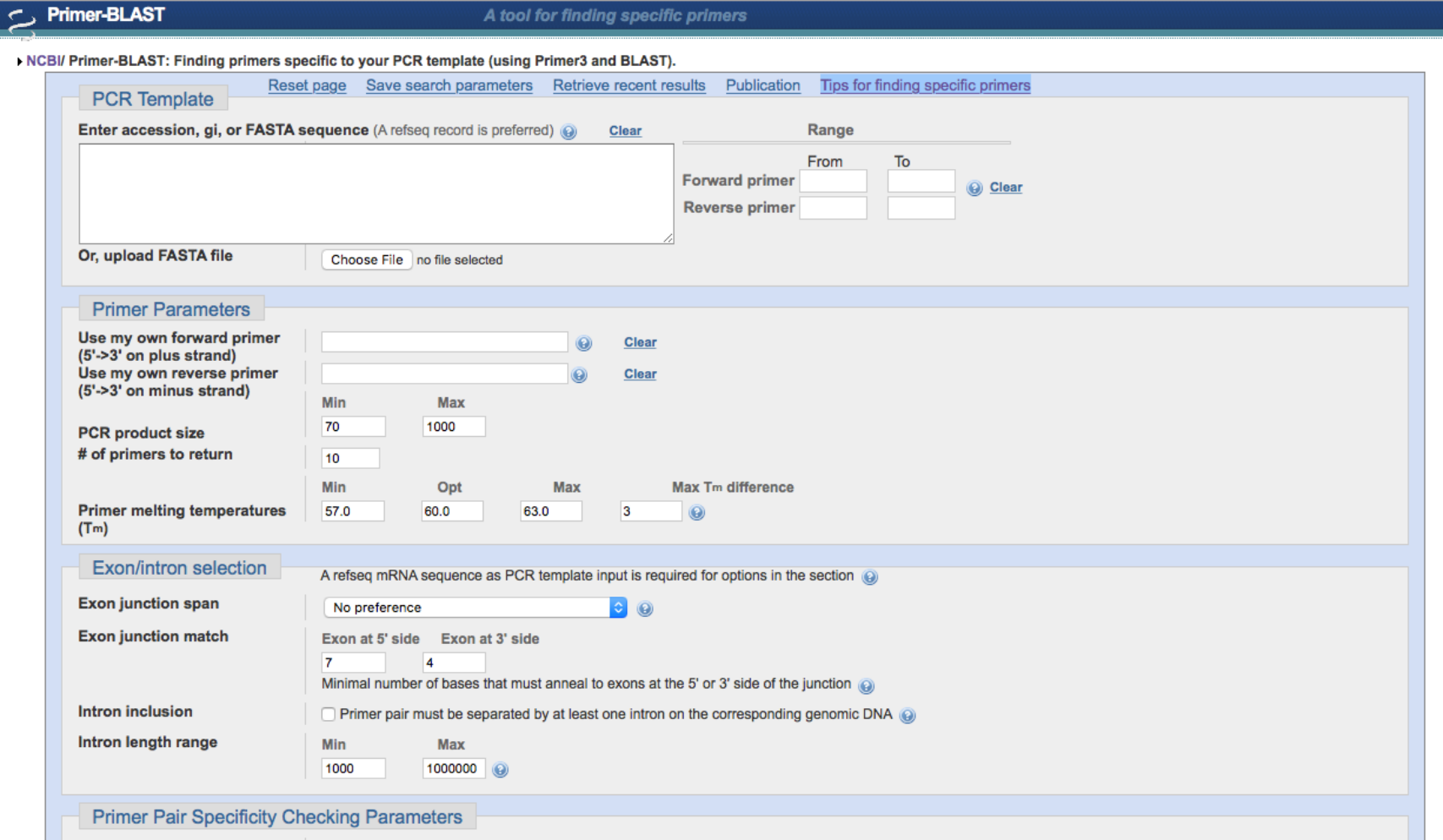
Download the genomic sequence of the Avr1 gene locus from BrightSpace. To help you design ‘appropriate’ primers (remember what characteristics are important when designing a primer), we will use PrimerBLAST. PrimerBLAST combines Primer3, a program that designs primers for a given target sequence, and BLAST, which determines if the primer sequences are specific.
Have a look at the settings for the expected product size (default value is set to be between 70-1000nt). What does this mean?
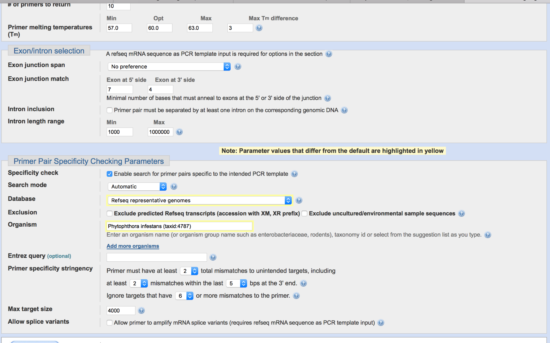
We want to make sure that our designed primers are as specific as possible. Therefore, we want to avoid that the designed primer can match to any other region in the genome other than the target region, in this case Avr1. Therefore, we can indicate that PrimerBLAST will check the specificity against the P. infestans genome sequence. To this end, select the database (‘Refseq representative genomes’) and enter Phytophthora infestans in the ‘organism’ field. One of the possibilities is also to use the ‘non-redundant’ (nr) database. Can you imagine why choosing the nr database can be a problem when identifying specific primer sequences?
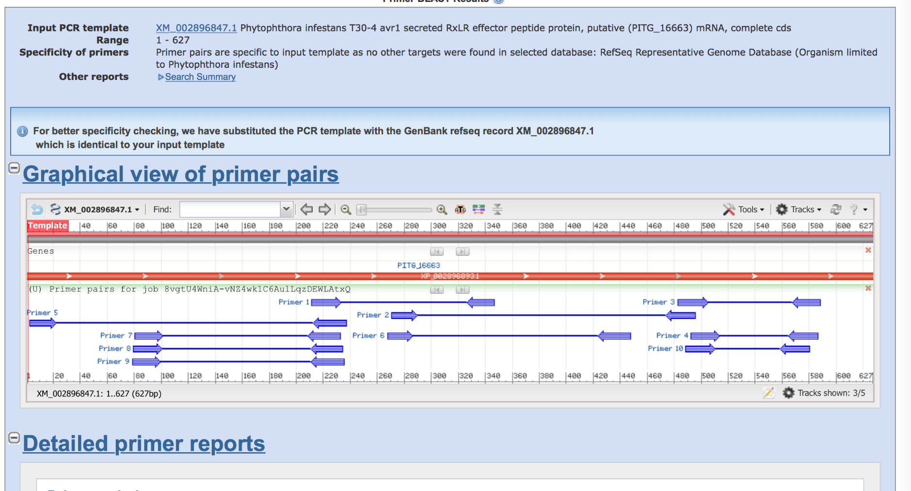
Enter the sequence of Avr1 into the search field of PrimerBLAST, and run PrimerBLAST with the options defined under question 3 (database and organism). PrimerBLAST will identify that your Avr1 is matching to an existing sequence in the database, which can interfere with the identification of specific primers. To make sure that PrimerBLAST takes this into account, select the database sequence, and proceed by clicking on the submit button.
Look at the results from PrimerBLAST. On top, you will find a summary about your submitted sequence (its length), and a message on whether PrimerBLAST was able to identify specific primers. Below, you will find a graphical overview of the distribution of the primer pairs along your sequence, as well as detailed information for each of the primer pairs (e.g. GC, Tm, length, and product length). Which of the primer pairs would be the best, and why (clearly all primers fulfill the quality criteria)?
If you place your mouse over the primer pair in the graphical overview, you can save the sequence of the primer and the product as a FASTA formatted file. Moreover, you can also directly search the product to the NCBI databases using BLAST. Why is it useful to save such a primer sequence?
BLAST the product of ‘Primer pair 1’, set the Max target sequences to the maximum and leave all other settings to default. How many hits do you find in the database that match your product? Can you imagine why PrimerBLAST indicated that your primer pair is specific?
PCR cannot only amplify regions from the genome, but also regions from mRNA (mRNA needs to be first converted into cDNA). When performing this type of PCR, one tries to design primer pairs that span an intron in the gene of interest (this is also an option in PrimerBLAST). Can you speculate why primers spanning an intron can be helpful?
Assignment VIII answers
PrimerBLAST looks very similar to other blast tools, and thus you should feel familiar by now.
The expected product size indicates the size of the PCR product to be amplified by the designed primers; normally, you want to have products around 250-400 nt for PCR and ~150 for qPCR; longer fragments are more challenging and require optimization of run times and components.
Exclusion and specific sequences can be utilized similarly to normal blast. Using nr is not advised as even though the db is non-redundant, there are often highly similar matches from other species/strains/cultivars that might indicate non-specific binding for the target organisms interested.
PrimerBLAST is able to help you to overcome issues with identical sequences being in the database. If PrimerBLAST would not do so, every search would likely return a non-specific primer pair.
All primers are okay (based on the defined parameters). The ideal product length for DNA is in the range 150-1000bp (in practice 150-300bp is used a lot, but it depends on the purpose of the PCR). For example, primer pair 2 (225 bp product) or 7 (152 bp product) would be good.
Saving the primer is relevant as these sequences can be used to order primers.
135 hits are found in the nr database. Interestingly, the first four matches in the database are all 100% identical matches of the input product. Number four is the strain we started with, but apparently there are three other strains for which this piece of DNA is identical. PrimerBLAST still indicated that the primer is specific, because there is only one exact copy of this piece of DNA in the genome. There is actually a hit on the same strain (T30-4), but in a different sequence. However, this hit has some mismatches in the location where the forward primer hybridizes, so likely there will be no amplification.

mRNA is first converted to cDNA as RNA and DNA will not hybridize well; Designing over an intron allows to distinguish PCR products from genomic DNA or cDNA (as cDNA does not contain the introns); cDNA is typically shorter and will run at different height.
Project Preparation Exercise
We continue the project exercise from chapter 1. Both ARF5 and IAA5 belong to large gene families in A. thaliana. Now, focus on the ARF5 family and explore it by identifying homologs and looking for conserved parts among the family members. Perform this analysis both within Arabidopsis thaliana and outside of this species. Assess in which plant families members are detected.
Describe the following items in a few bullet points each. You may include up to two figures or tables.
Materials & Methods What did you do? Which data, databases and tools did you use, and why did you choose them? What important settings did you select?
Results What did you find, what are the main results? Report the relevant data, numbers, tables/figures, and clearly describe your observations.
Discussion & Conclusion Do the results make sense? Are they according to your expectation or do you see something surprising? What do the results mean, how can you interpret them? Do different tools agree or not? What can you conclude? Make sure to describe the expectations and assumptions underlying your interpretation.
References#
- 2W1(1,2,3,4,5,6,7,8,9,10,11,12,13,14)
Dick de Ridder, Anne Kupczok, Rens Holmer, Freek Bakker, Justin van der Hooft, Judith Risse, Jorge Navarro, and Tomer Sardjoe. Self-created figure. 2024.
- 2W2(1,2)
Thomas Junier and Marco Pagni. Dotlet: diagonal plots in a web browser. Bioinformatics, 16(2):178–179, 02 2000. URL: https://doi.org/10.1093/bioinformatics/16.2.178, arXiv:https://academic.oup.com/bioinformatics/article-pdf/16/2/178/48835958/bioinformatics\_16\_2\_178.pdf, doi:10.1093/bioinformatics/16.2.178.
- 2W3(1,2,3)
Fábio Madeira, Matt Pearce, Adrian R N Tivey, Prasad Basutkar, Joon Lee, Ossama Edbali, Nandana Madhusoodanan, Anton Kolesnikov, and Rodrigo Lopez. Search and sequence analysis tools services from embl-ebi in 2022. Nucleic acids research, 50(W1):W276—W279, July 2022. URL: https://europepmc.org/articles/PMC9252731, doi:10.1093/nar/gkac240.
- 2W4
Ppgardne. Blosum62-dayhoff-ordering. 2022. URL: https://commons.wikimedia.org/wiki/File:Blosum62-dayhoff-ordering.svg.
- 2W5
National Library of Medicine (NLM). How blast works. 2022. URL: https://www.nlm.nih.gov/ncbi/workshops/2022-10_Basic-Web-BLAST/how-blast-works.html.
- 2W6
Christiam Camacho, George Coulouris, Vahram Avagyan, Ning Ma, Jason Papadopoulos, Kevin Bealer, and Thomas L Madden. Blast+: architecture and applications. BMC Bioinformatics, 10:421, dec 2009.
- 2W7
Kazutaka Katoh and Daron M. Standley. MAFFT: Iterative Refinement and Additional Methods. In David J Russell, editor, Multiple Sequence Alignment Methods, pages 131–146. Humana Press, Totowa, NJ, 2014. doi:10.1007/978-1-62703-646-7_8.
- 2W8
Randall K Saiki, Stephen Scharf, Fred Faloona, Kary B Mullis, Glenn T Horn, Henry A Erlich, and Norman Arnheim. Enzymatic amplification of β-globin genomic sequences and restriction site analysis for diagnosis of sickle cell anemia. Science, 230(4732):1350–1354, 1985.
- 2W9
National Human Genome Research Institute (NHGRI). Pcr reaction. 2024. URL: https://www.genome.gov/genetics-glossary/Polymerase-Chain-Reaction.