
3. Phylogenetics and tree reconstruction#
– Freek T. Bakker
In this chapter you will learn to use a Multiple Sequence Alignment (MSA), like the ones you compiled in chapter 2, and visualize the variation it contains as a phylogenetic tree. A phylogenetic tree is considered a highly efficient data structure summarizing the data and its variation contained in your MSA. A tree is built from characters which are the individual columns or positions in your MSA. Characters have states, which are in this case the individual nucleotide or amino acid substitutions occurring in that position (see Characters & trees below). Invariable characters are columns or positions ‘occupied’ by just one type of nucleotide or amino acid, whereas variable characters may have up to 4 different nucleotides or up to 20 amino acids per position.
DNA and amino acid (AA) sequences contain the information necessary for building protein structure, comparing them in an MSA will enable insight how these structures, and their associated functions, may have changed over evolutionary times since they descended from an ancestral sequence. The more character state changes (i.e., substitutions) occur between sequences, the more diverged they are and probably also less related (see Related, diverged below), and hence the further apart they will occur on your phylogenetic tree. The information contained in your tree is hierarchical in nature, meaning that it is built-up as nested sets of subtrees that are also known as clades. A clade is a group containing an ancestor together with all its descendants and is also referred to as a monophyletic group.
Rationale#
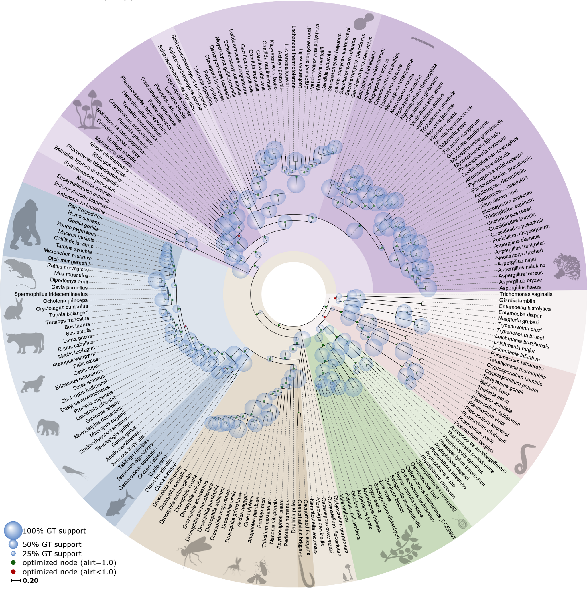
Fig. 3.1 Simplified Tree of Life. Credits:
CC BY 4.0 [Huerta-Cepas et al., 2014].#
Why should we study phylogenetics and what is it about? Ever since Darwin we know that all living things are connected in a tapestry of life, forming a phylogenetic tree of everything (Fig. 3.1). Phylogenetics aims at understanding evolutionary relationships among genes, species, and higher taxa and as such it is relevant to almost all biological questions. Why? Because an evolutionary context (rather than a ‘snapshot’ perspective) allows identifying evolutionary lineages and their origins, and can provide information on how lifeforms and sequences change and adapt across millions of years. Examples are studying the evolution of gene families within genomes, or the build-up of species relationships in a lineage.

Fig. 3.2 The SARS-CoV-2 phylogenetic tree, March 2024. Credits: CC BY 4.0 [Hadfield et al., 2018].#
Other examples are studying Covid-19 and other pathogen outbreaks (Fig. 3.2), studying molecular evolution and the accumulation of substitutions in a multiple sequence alignment (MSA). Or, studying population history within a species, reconstructing historical biogeography: In all these cases having an accurate phylogenetic tree is crucial, because we want to be able to reconstruct evolutionary lineages (the branches in phylogenetic trees) and how they evolved, changed, duplicated, or went extinct. By accurate we mean estimating relationships that are as close as possible to the actual (historic) relationships, which we cannot know for sure. As they happened in the past we cannot prove them, but they are hypotheses (of relationships) that we can only corroborate (confirm, seek support for).

Fig. 3.3 Comparing species (or genes) in a phylogenetic tree allows inference of ancestral states and evolutionary trends. Credits: CC BY-NC 4.0 [Ridder et al., 2024].#
When a phylogenetic tree is known for a specific group, and it is properly rooted, the ancestral states for its characters can in principle be reconstructed (for instance the ancestral amino acid residues in a protein sequence) for each node in the tree. With that, evolutionary trends (towards current conditions) can be inferred, enabling the study of character evolution, i.e., how things change over time (Fig. 3.3).
Phylogenetic trees: structure & interpretation#
Like all trees, phylogenetic trees come with a stem, branches, leaves and ideally a root. What makes phylogenetic trees special however is that they are actually hypotheses of evolutionary relationships, as outlined in the previous section. The leaves or external nodes are then the individuals (or sequences) that are observed and compared, which are also referred to as operational taxonomic units (OTUs) or terminals. The branches and nodes are the lineages or clades that are inferred, i.e., not observed. A clade is an ancestral node together with all its descendants, which is also referred to as a monophyletic group. They are recognised by the horizontal lines connecting the OTUs and HTUs (hypothetical taxonomic units) in your phylogenetic tree, as for instance shown in Fig. 3.4.
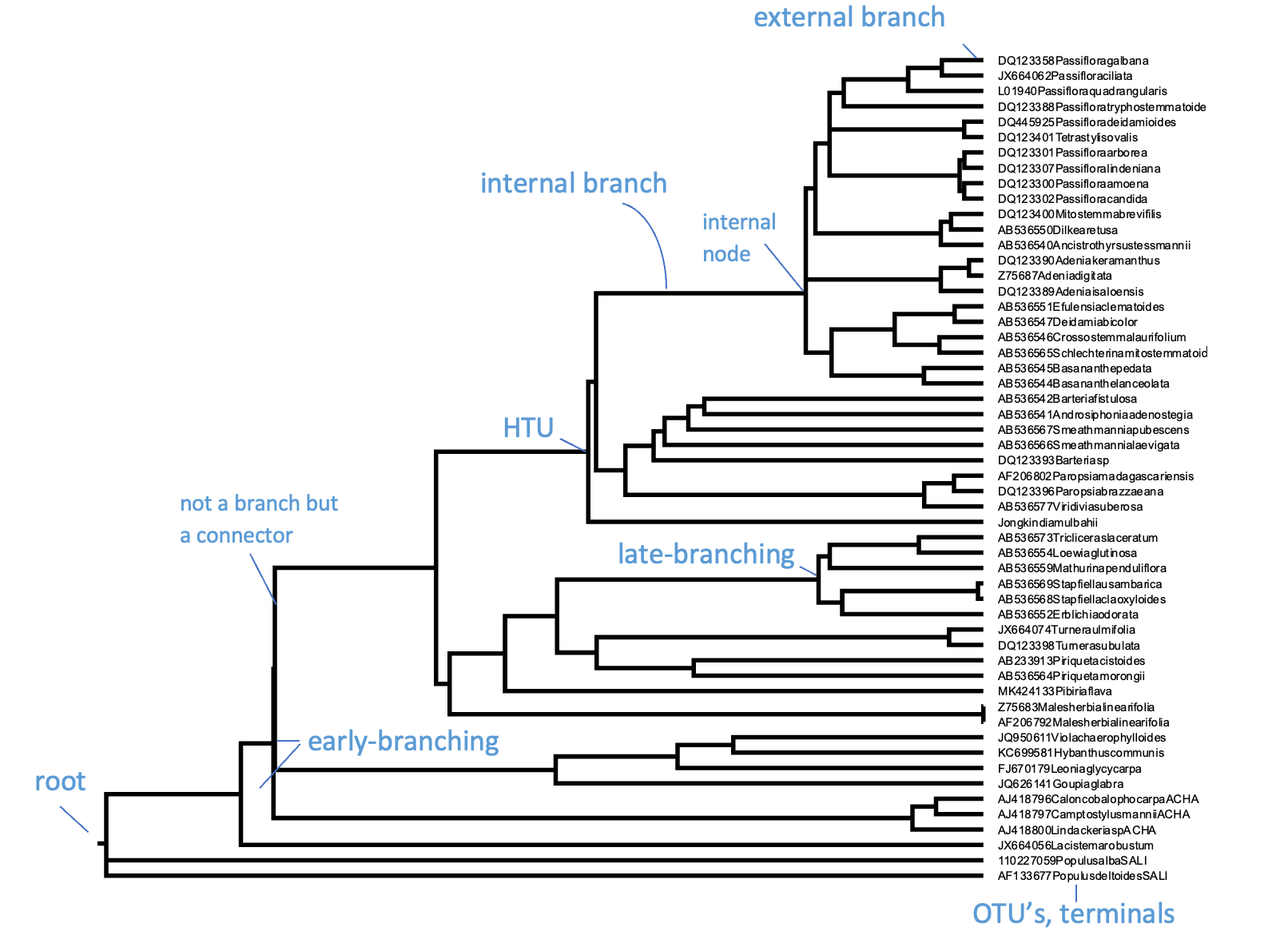
Fig. 3.4 A rooted ultrametric phylogenetic tree with its main parts and characteristics indicated. Here, the OTUs are GenBank plant chloroplast gene accessions, the names of which have been condensed. Credits: CC BY-NC 4.0 [Ridder et al., 2024].#
Whereas the horizontal lines represent the actual branches, the vertical lines do not have a meaning and are just there to connect the branches and clades; they will get longer when more terminals are included but do not have a relation with the data (i.e., the MSA). Branches are connected via nodes, that can be internal (HTUs) or external (OTUs). Internal nodes represent hypothetical ancestors that are not observed or sequenced but inferred or reconstructed. As outlined above, external nodes are the actual individuals observed; they are never connected directly to each other, only through internal nodes. These individuals can represent genes, species or higher taxa, but they are never categories (or averages), as characters and states are indivisible observations scored on individuals. Branches and nodes collectively build the tree topology, i.e., the structure of the tree.
One of the most important aspects of a phylogenetic tree is whether it is rooted, meaning whether we can distinguish which nodes are old and which are more recent, and also what clades are present. Rooting is done by selecting an outgroup, which is a reference taxon outside the group of interest (this is described in more detail in section Rooting & clades). It is important to realise that most phylogenetic reconstruction methods actually produce unrooted trees, which can then rooted using an outgroup to visualize in what direction evolution proceeded and which clades can be identified.
Related, diverged#

Fig. 3.5 Additive phylogenetic tree of mammalian species, rooted on monkey. The MRCA of monkey, bear, seal and dog is indicated. Tree topology informs relatedness, branch lengths correspond to divergence. Credits: CC BY-NC 4.0 [Ridder et al., 2024]. Made using imagery from: CC BY 4.0 [DataBase Center for Life Science (DBCLS), 2023]#
In a rooted phylogenetic tree, terminals sharing a more recent common ancestor are more closely related than terminals sharing a less recent common ancestor. Thus, in Fig. 3.5, dog and bear are more related than dog and seal, because dog and bear share a more recent common ancestor. On the other hand, monkey and dog are as related as monkey and cat, because they all share the same most recent common ancestor (MRCA). Being related is not the same as being diverged, as divergence means the amount of change accumulated since the split of two lineages, which is reflected in the branch lengths (or in distances). In our example, raccoon and dog would be more diverged than raccoon and bear, but not more closely related.
Cladogram, additive and ultrametric#
Phylogenetic trees come in three flavors: ultrametric, additive, and cladogram. When all paths starting from the root to each external node are of equal length, you could interpret the length of a path through the tree as proportional to time and thus equally old as other paths; the ages of nodes can then in principle be inferred. Such a tree is known as an ultrametric tree, which can be easily recognised by its topology in which all terminal branches line up, usually to the right. Another, more common type of phylogenetic tree is the additive tree, in which branch lengths are proportional not to time but to the amount of change occurring in your data set (the MSA). Therefore, the more changes (i.e., substitutions, insertions, deletions) occur for an individual, the longer the branch to its MRCA will be in the additive tree. Most phylogenetic and tree building platforms or software packages produce additive trees. Producing ultrametric trees usually requires taking extra steps, with each step introducing uncertainty. You could argue that ultrametric trees are one extra step away from the data compared to additive trees. Only when the data accumulates substitutions in a strictly clock-like manner (i.e., like radio-active decay) would the ultrametric and additive tree version be the same. However, such strict molecular clocks are never encountered in real data. Finally, a cladogram-style tree is a ‘schematic tree’ meant to only show the topology of your tree. It therefore has artificial (equal) branch lengths, including for terminal branches.
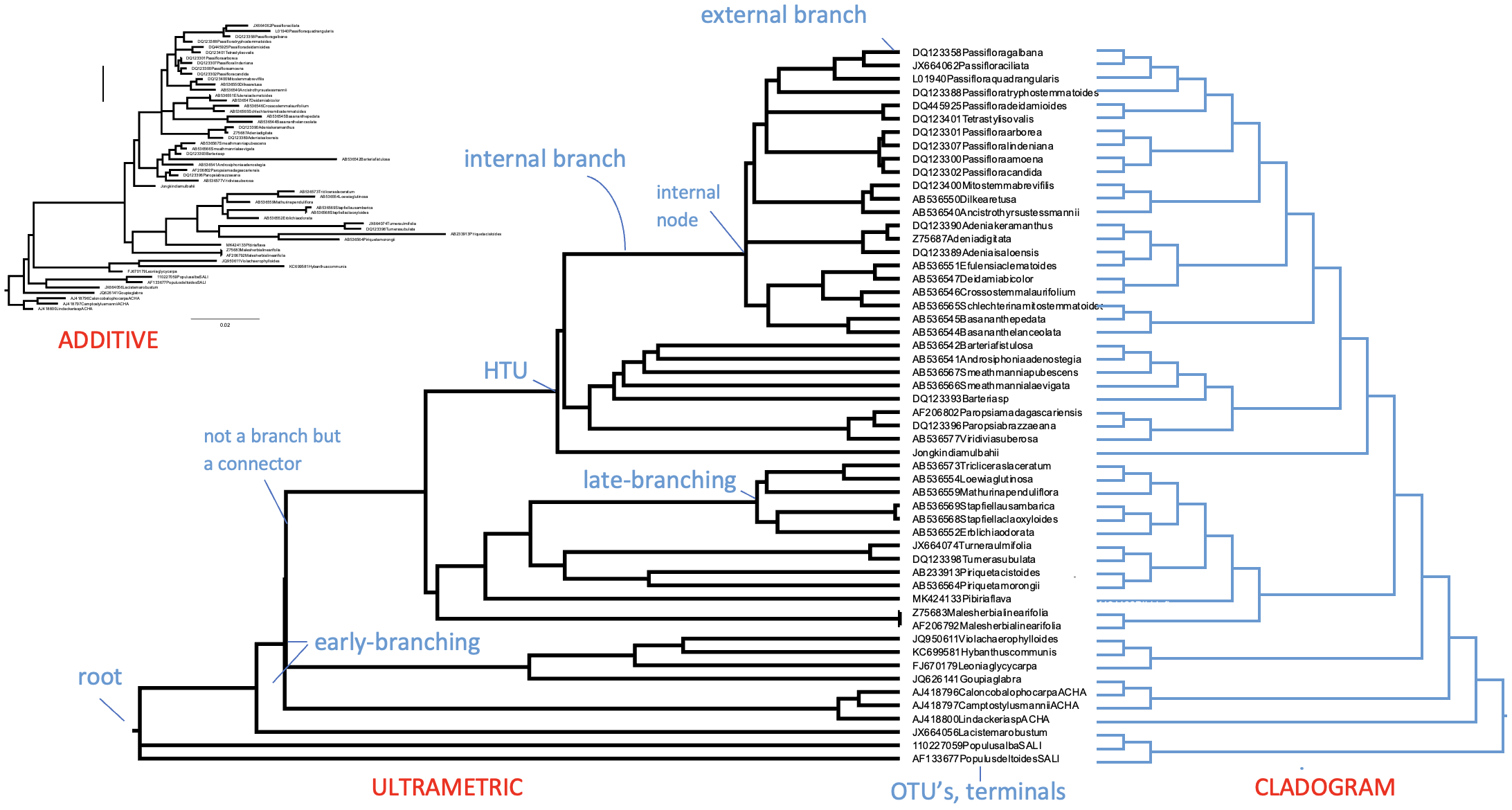
Fig. 3.6 A rooted phylogenetic tree with its main parts and characteristics indicated. Here, the OTUs are GenBank plant chloroplast gene accessions, the names of which have been condensed. For the same data, the tree is given as additive tree (top) and as an ultrametric tree (bottom left) with branch lengths corresponding to time. On the right, flipped, the same tree as cladogram, with branch lengths only indicating the structure of the trees.#
Tree resolution#
The resolution of a phylogenetic tree is the extent to which nodes and branches (clades) can be inferred/observed from the tree. Trees can be fully resolved, in which case each internal node is connected to three branches: the ancestral branch and two subtending branches. Such trees are called bi-furcating or dichotomous, meaning that each branch splits into two and there are no uncertainties on branching order or resolution of nodes. Frequently however, phylogenetic trees will be partly resolved and contain polytomies, which are nodes connected to (many) more than three branches. Polytomies represent parts of the phylogenetic tree that are uncertain in terms of branching order of the lineages involved. This can be due to there being insufficient information in the MSA for resolving the lineages, or ample but conflicting signal. Polytomies are usually interpreted as soft, meaning that the data used does not allow to resolve the lineages inferred (Fig. 3.7).

Fig. 3.7 Hard and soft polytomies in a phylogenetic tree. The soft polytomy can imply different tree resolutions. Credits: CC BY-NC 4.0 [Ridder et al., 2024].#
In contrast, the hard interpretation would be: instantaneous speciation, i.e., an ancestral species lineage split up so fast that the new lineages do not have sufficient unique substitutions to ‘mark’ them and to assign them an internal node in the tree. An example is the late-Tertiary radiation of mammalian orders, after the fairly quick establishment of cold water around the Earth’s poles, combined with that of the hot tropics. Several published mammalian phylogenetic trees contain unresolved spines or backbones.
On the other hand, gene trees (used for studying gene families) may also contain polytomies and they are usually considered as soft (the data is not decisive enough to infer a branching order). Whole genome duplications (auto-polyploidisations) are fairly well known, especially in the evolution of flowering plants. Following such an event, pairs of genes can be expected to form instantaneously, i.e., without accumulating unique substitutions, and may result in hard polytomies in gene trees.
Orthologs & paralogs#
When the terminals included are actually gene or protein sequences, the tree will be a gene tree, likely containing homologs (derived from a common ancestor gene), possibly also orthologs and paralogs. Orthology is the occurrence of corresponding, homologous (and mostly similar), genes in lineages resulting from speciation. For instance, human beta globin and chimp beta globin are orthologs. Usually, these genes will have the same function in different species, but this doesn’t necessarily have to be the case. In contrast, paralogy is the occurrence of similar genes resulting not from speciation but from gene duplication. For example, proteins from a gene family with different functions in the same species. Such similar genes are referred to as paralogs, which are visualized as multiple occurences of particular terminals on the tree. Fig. 3.8A and B illustrates the process of gene duplication followed by speciation, resulting in two parallel subtress (the grey X tree and the green X’ tree). Fig. 3.8C shows the challenge with using both orthologs and paralogs in phylogenetic analysis when not all members of a gene family have been sampled.

Fig. 3.8 The challenge of paralogs: (A) Paralogous genes are created by gene duplication events. Gene X is duplicated in a (recent) common ancestor (RCA) of species A and B resulting in paralogous genes X and X’. Species A and B inherit both copies of the gene (unless one or the other is lost somewhere along the way). (B) Phylogenetic analysis of the X/X’ gene family gives two parallel phylogenies. All sequences of gene X are orthologues of each other, as are all sequences of gene X’. However, X and X’ are paralogues. Both the X and X’ subtrees show the true relationships among the three species. The subtrees are also each other’s natural outgroup, and as a result each subtree is rooted with the other (reciprocally rooting). (C ) A tree of the X/X’ gene family can be misleading if not all the sequences are included (because of incomplete sampling or gene loss). If the broken branches are missing, then the true species relationships are misrepresented. Credits: CC BY-NC 4.0 [Ridder et al., 2024].#
In Fig. 3.9, a sequence of events is given involving two duplications and one speciation event that can lead to a set of homologous genes in two species. Some of these are orthologs and some are paralogs that have acquired new functions. A species tree is depicted by the pale blue cylinders, with the branch points (nodes) in the cylinders representing speciation events. In the ancestral species (on top) a gene is present as a single copy and has function α (blue). After some time, a gene duplication event occurs within the genome, producing two identical gene copies, one of which subsequently evolves a different function, identified as β (red). As a result, α and β are now paralogous genes. Later on, a speciation event occurs resulting in two species (A and B), both containing genes α and β. Gene Bα (in species B) subsequently undergoes another duplication event, resulting in the paralogous genes Bα and Bγ. After further divergent evolution, Bγ, aquires a new function γ (green). The Bα gene is still functionally very similar to the original gene α. At the end of this period of evolution, all five genes in the two species are homologous, with three orthologous pairs: Aβ/Bβ, Aα/Bα, and Aα/Bγ. The Bα and Bγ genes are paralogous, as are any other combinations except the orthologous pairs. Note that Aα and Bγ are orthologs despite their different functions. The gene tree inferred from these five genes has multiple occurrences of both species A and B (Fig. 3.9B).

Fig. 3.9 The evolutionary history of a gene that has undergone two separate duplication events. (A) The species tree (large blue cylinders) comprising species A and B and with indicated gene duplication and neo-functionalisation events leading to β and γ functions. (B) The phylogenetic tree that would be drawn for the resulting 5 genes in (A), here drawn as a cladogram. Credits: CC BY-NC 4.0 [Ridder et al., 2024].#
For another example of a gene versus species tree consider the trees in Fig. 3.10, which are based on the comparison of Interleukin gene sequences. There are multiple occurrences of the terminals from the species tree (bovine, sheep, pig etc.) in the gene tree, each grouped with a different Interleukin sequence type. These are the paralogs, that probably resulted from gene duplication events during the proliferation of the IL clade.
Given that there are four copies of IL1 in humans (indicated with green boxes in the gene tree in Fig. 3.10), there must have been at least three gene duplications in the history of the interleukins. Three of them are inferred from the presence of multiple copies of IL in the same mammalian species, i.e. i) in the ancestor of the IL-1α + β clade, ii) in the ancestor of the IL-1rα + β clade, and iii) as a sister pair in the IL-1β clade. Duplication δ3 is required to explain the incongruence between the mammalian species tree and the IL-1β phylogeny. The incongruence is that in the gene tree human and mouse are more closely related than either is to bovine/sheep. The species tree however indicates human to be more closely related to bovine/sheep than to mouse. In order to resolve (reconcile) this, δ3 is suggested as indicated in Fig. 3.11.

Fig. 3.10 A species tree based on external evidence (left) and a gene tree based on a comparison of mammalian Interleukin-1 genes (right). In the gene tree, both alpha and beta copies can be seen, which are probably the result of gene duplications (see Fig. 3.9). Occurrences of ‘Human’ in the gene tree are indicated with green boxes. Credits: CC BY-NC 4.0 [Ridder et al., 2024]. Made using imagery from: CC BY 4.0 [DataBase Center for Life Science (DBCLS), 2021].#
The tree in Fig. 3.11 is a so-called reconciled tree, which has been inferred as an extended tree that would be necessary to assume in order to explain the position and distribution of all IL sequence types in the gene tree. Apart from four gene duplications (marked δ1, δ2, δ3 and δ4), several gene losses (indicated with light grey branches) too would need to be assumed to explain the pattern in the gene tree in Fig. 3.10.

Fig. 3.11 Reconciled tree for the mammalian interleukin-1 gene tree shown in Fig. 3.10. Gene losses are indicated in light grey. Of the four duplications required, three are supported by the presence of multiple copies of IL in the same mammal species, and one (δ3) is required to explain the incongruence between IL-1 and mammalian phylogeny. Credits: CC BY-NC 4.0 [Ridder et al., 2024].#
Box 3.1: Species tree estimation analysis.
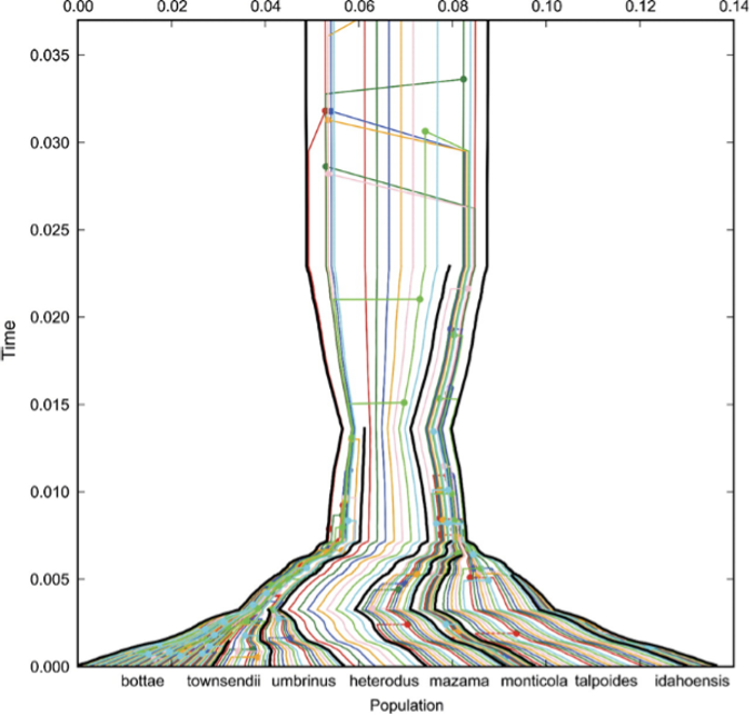
Fig. 3.12 Gene trees, in color, embedded in the
species tree (black lines) of western
pocket gophers (Geomyidae, Thomomys).
Credits: CC BY-NC 2.5
[Heled and Drummond, 2009].#
When terminals are individuals meant to represent species, we would in principle be inferring a species tree. Fig. 3.12 shows an example of multiple gene trees (in color) contributing to the species tree (indicated by black lines) as a result of species tree estimation analysis. The different species names, in this case Thomomys ‘Western pocket gophers’ (Geomyidae), are indicated along the horizontal axis and their coalescence (gene lineages coming together, looking backwards in time) can be traced through time. Such analysis is beyond the scope of this course, but it is of course important to always keep in mind at what level your phylogenetic reconstruction is, whether at the species, gene, or even biogeographic area level.
Nodal support in phylogenetic trees: the bootstrap#
Not all parts of a phylogenetic tree will be equally well-supported or strong, given our character data (MSA). There can be considerable uncertainty around the estimated nodes of our tree, affecting the confidence we have in those nodes. In experimental science, usually some statistic measure is used to quantify uncertainty, for instance the mean and standard deviation of outcomes of repeated experiments. Phylogenetics, however, is not experimental but rather seeks to reconstruct historic patterns that were driven/shaped by evolution. As outlined at the beginning of this chapter, the implication is that we cannot prove phylogenies, nor repeat them, or even know whether we reconstructed the correct one. We ‘only’ have our phylogenetic trees as estimates of the true phylogeny.
In order to measure support for the nodes in our phylogenetic tree, rather than producing several replicates of our MSA (which will most likely all be identical), we can draw random samples from the MSA and use these pseudo-replicate data sets to build trees (Fig. 3.13). Repeating this process many times (hundreds or thousands) and summarizing the variation among the trees thus reconstructed, provides insight in the structure of our data and how it supports the nodes in a tree. It actually measures the sampling variance about the estimate of the phylogeny Fig. 3.13B. This process is called bootstrap analysis and will be further discussed in Maximum likelihood tree building, after we have covered the characters underlying our trees in the next section.

Fig. 3.13 Bootstrap resampling analysis in phylogeny reconstruction. In case of unlimited data (A), not realistic, a summary of sample-based trees yields sampling variance about the true phylogeny. In case of limited data (B), realistic, only pseudo-samples are available, that summarise sampling variance about the estimate of true phylogeny. Credits: CC BY-NC 4.0 [Ridder et al., 2024].#
Characters & trees#
As outlined above, phylogenetic trees are not directly observed but inferred, and represent hypotheses of evolutionary relationship, grouping individuals on the basis of shared history. The data used for comparison are the homologous sites among a set of sequences (amino acid or nucleotide) that have been aligned in an MSA in which substitutions are made visible. Homologous here means that there are corresponding positions in a gene sequence that are due to common ancestry. So, for instance, position 423 in a gene sequence from one species is homologous with position 423 in that of another species, because both species shared a recent common ancestor and we assume the genes to be orthologs. Each such position is considered a character with states that are efficiently visualized in an MSA as substitutions (Fig. 3.14A). All nucleotide or amino acid substitutions in the MSA, both unique ones (occurring in only a single individual or sequence) and shared ones (occurring in at least two sequences), are used to build the phylogenetic tree. Invariant characters however, showing no substitutions, are not expected to contribute to the tree building process as they do not contain comparative signal. Shared substitutions are informative for building the branches of your tree, as they group terminals and hence add to the length of internal branches. Unique substitutions on the other hand only contribute to the twigs or external branch lengths and have no grouping power. The more shared substitutions occur for a set of sequences in your MSA, the stronger the resulting node in the phylogenetic tree will be supported.

Fig. 3.14 Characters and trees. A: Multiple sequence alignment (MSA, nucleotides) with examples of shared-derived (S), unique (U) as well as invariant (I) characters indicated; B: MSA containing S, U and I characters and the number of steps per character, as well as the total tree length for tree1 and tree2 indicated on the bottom lines.; C: two ‘candidate trees’ as alternative hypotheses explaining the data in the MSA in (B), with character state changes for all characters are indicated on the trees and exemplar syn- and autapomorphies are indicated. Note that character 6 is invariant and therefore does not contribute to any tree. Tree 1 requires one step less than tree2 and is therefore the preferred tree. Credits: (A) created using MEGA11 and modified from [Tamura et al., 2021] (B & C) CC BY-NC 4.0 [Ridder et al., 2024]#
When observing substitutions in an MSA we cannot say which ones are ancestral (occurring already in ‘deep’ ancestors) and which ones are derived, occurring more recently. But placed in the context of a rooted phylogenetic tree, shared substitutions can actually be shared derived substitutions, which are known as synapomorphies (syn=shared, apo=derived, morphy=character), whereas uniquely derived substitutions are called autapomorphies (see Fig. 3.14B & C).
When designing a phylogenetic study, involving the compilation of one or more MSAs, there is usually a choice between adding more characters (lengthening the MSA) versus adding more terminals (adding more sequences(rows) to the MSA). Whereas the former is tempting, it is often more useful to add terminals (taxa) as this allows extra synapomorphies to be realised. After all, synapomorphies are relative (not absolute) entities: only in the context of other sequences can you actually ‘see’ them. For instance, when studying a gene family in which duplications have occurred during the evolution of its lineages, many taxa should be included in the MSA in order to capture the duplication events. Only adding more characters may amplify errors or artefacts caused by taxic under-sampling. This can lead to incorrectly inferred long branches with seemingly high support for their position and nodes. This phenomenon is referred to as long-branch attraction and is discussed further in Estimating sequence divergence.
Rooting & clades#
A clade is an ancestral node together with all its descendants, which is also referred to as a monophyletic group. We usually refer to the ancestral node of a clade as the inferred most recent common ancestor (MRCA). Of course, there will always be less recent (‘deeper’) ancestors but they will probably not be informative for recognising and inferring a clade and its relationships, as they are also the ancestor of other clades. At deep divergences (e.g., herring versus fruit fly), homology and resolution of the characters used may not be clear and sufficient.
Information contained in phylogenetic trees is hierarchical, with structures being part of other, more inclusive, ones. Clades are indeed usually nested into each other, i.e., a clade is a subset of a larger clade. Apart from being nested, clades can also be each other’s sisters, which means they share an exclusive most recent common ancestor (MRCA) with no other clades included (Fig. 3.15). Such sister groups are highly useful in, for instance, evolutionary and comparative studies, as they represent lineages of exact equal age.

Fig. 3.15 Nested clades and sister clades. Top, the same rooted tree as in Fig. 3.16, now with nested clades indicated with orange and green shapes: the small orange clade is nested in the larger -dashed- one; it is also a sister clade of the green clade; as are the blue and larger dashed clades. Bottom, nested and sister clades with MRCA indicated. Credits: CC BY-NC 4.0 [Ridder et al., 2024].#
Again, an MRCA together with all its descendants is considered to form a clade. Such a clade can then be the basis of further analysis or classification. It is good to realise that the clade is based on observations (synapomorphies) and therefore represents evidence, whereas classification is in principle subjective (opinion) and an interpretation and use of the clade. For instance, when any descendant of a clade is left out in a classification, for example Vertebrates being left out from the Invertebrates, or birds left out from dinosaurs, the proposed taxon or classification is not monophyletic anymore and is considered a paraphyletic group (i.e., an MRCA and not all its descendants). Paraphyletic groups (also referred to as non-natural groups) are still in use but not considered to be a proper basis for classification.
When studying gene families and their evolution, it is useful to make comparisons among clades in the gene tree, especially among sister clades, as they are of exactly the same age. Any differences between them, in terms of substitution rates, sequence bias in composition, or the number of lineages per clade, is then due to speciation processes, not the different age of the clades. In order to make these comparisons it is important to compare monophyletic and not paraphyletic groups as the latter are not directly comparable or of equal age.
Rooting a tree is polarising it, making a distinction in what are old and younger nodes. When a tree is properly rooted, usually with an outgroup reference taxon outside the group of interest, it is therefore directed in terms of ancestry and clades can be inferred (see Fig. 3.16B; Note that unrooted trees, which are non-polarised, in principle do not contain clades but ‘clans’). In the example in Fig. 3.16, B, we see that the rooted version of the bird phylogenetic tree seems to contain one extra brown bird. External evidence (which is not shown in the figure, only the vertical branch on top leading to the outgroup) was apparently convincing in placing the root between the white and brown birds. Thus, a new, internally placed, brown bird is inferred as the MRCA, to which the outgroup branch can attach. This however makes the brown birds paraphyletic with regards to the white birds, because not all descendants from the brown MRCA are brown, some are white. The white birds themselves are now monophyletic.

Fig. 3.16 Rooting phylogenetic trees. (A) Unrooted tree depicting phylogenetic relationships among a set of white and brown bird species; external nodes represent the extant (living, observed) species, each with their morphological synapo- or autapomorphies, the internal nodes represent inferred (unobserved) ancestors. The tree is fully resolved, as each internal node is connected to three branches. Looking at the brown and white birds at adjacent internal nodes, it is not clear in what direction evolution proceeded and whether brown yielded white or rather the other way round. This becomes possible upon rooting the tree, usually based on comparison with an external reference species. (B) Rooted tree; external evidence (not shown) was apparently convincing in placing the root between the white and brown birds. Thus, a new, internally-placed, brown bird is inferred as the MRCA, making the brown birds paraphyletic with regards to the white birds, which are now monophyletic. Credits: CC BY-NC 4.0 [Ridder et al., 2024]#
Improper rooting affects clades and the overall structure of tree (as illustrated in Fig. 3.17). The correct rooting of this tree is indicated, with human and chimpanzee as sisters, which is undisputed and based on external evidence for these species. Placing the root at the seven possible different positions in the unrooted tree of five terminals shows that only in three cases the (correct) human-chimp-gorilla monophyly is maintained (Fig. 3.18). The other four topologies show extensive conflict, both with each other and with the correct topology. This indicates that care should be taken in selecting and assigning a suitable outgroup, which can be problematic in the case of isolated long phylogenetic branches (for instance, in protists or zooplankton lineages) or in the case of reconstructing a gene tree. In that case, one usually considers a copy of the gene of interest with sufficient similarity to be considered homologous, in a far-related evolutionary lineage (such as Amborella, for angiosperm plants) as a suitable outgroup for rooting that gene tree. Fig. 3.19 shows an example of an unrooted tree with additive branch lengths.

Fig. 3.17 Rooting phylogenetic trees. With human (H), chimp (C ), gorilla (G), orang-utan (O) and gibbon (B) indicated, the rooted tree (top) represents the correct tree topology based on external evidence. The position of this root is indicated, both in the rooted and unrooted tree. Credits: CC BY-NC 4.0 [Ridder et al., 2024].#

Fig. 3.18 Rooting phylogenetic trees. The seven rooted trees that can be derived from the unrooted tree for five sequences in Fig. 3.17. Each rooted tree 1-7 corresponds to placing the root on a different branch of the unrooted tree. Terminal labels as for Fig. 3.17; the orange shape indicates monophyly of human, chimp, and gorilla, when present. Credits: CC BY-NC 4.0 [Ridder et al., 2024].#

Newick tree notation#
Phylogenetic trees are graphical structures (‘graphs’) that are the outcome of phylogenetic reconstruction of sometimes hundreds or thousands of sequences, and especially when using character-based tree search (see below Main approaches to tree building) there can be enormous amounts of ‘best trees’ that all will have to be taken into account, for instance by calculating a consensus tree (see Tree space and heuristic search methods).
In any case, handling large numbers of trees in phylogenetical and bioinformatic analytical pipelines requires the tree graphs to be in a format that can be easily read and produced, as a linear statement.
For this, the Newick notation is commonly used in which brackets describe the structure of the tree.
For instance, the rooted tree in Fig. 3.17 above would look like ((((H,C)G)O)B) in Newick notation.
In case the tree has branch lengths, they can be indicated in this notation as well (see also the Newick tree Activity suggested on Brightspace).
Box 3.2: Newick notation tree reconstruction.
(Photobacterium_profundum:0.0713485869,Vibrio_cholerae:0.0572857616,(((((Coxiella_burnetii:0.0942829505,(((((Bartonella_henselae:0.0149660313,Bartonella_quintana:0.0104976443)100:0.0417236852,(Bradyrhizobium_japonicum:0.0661124319,Brucella_melitensis:0.0305911464)84:0.0159603838)100:0.0717972517,Caulobacter_crescentus_CB15:0.1317093492)89:0.0321405560,((Rickettsia_prowazekii:0.0221103197,Wolbachia_pipientis:0.0257883738)76:0.0009060796,Rickettsia_conorii:0.0023047443)100:0.1908928012)100:0.1212044773,((Campylobacter_jejuni:0.1640483645,(Helicobacter_pylori:0.0777846753,Helicobacter_hepaticus:0.0262963532)97:0.0750887828)100:0.3046033428,((Geobacter_sulfurreducens_PCA:0.0953158405,Desulfovibrio_vulgaris:0.2786904064)52:0.0512359438,Bdellovibrio_bacteriovorus:0.2548155296)65:0.0488493427)81:0.0360783687)100:0.0960879477)74:0.0330231208,((Xylella_fastidiosa_9a5c:0.0356264562,Xanthomonas_axonopodis_pv._citri:0.0296447972)100:0.0938726215,(((Bordetella_parapertussis:0.0000025222,Bordetella_pertussis:0.0033397334)100:0.0907958037,Ralstonia_solanacearum:0.0732876166)100:0.0326570294,(Chromobacterium_violaceum:0.0690355638,Neisseria_meningitidis:0.1027698727)75:0.0194002885)100:0.1171829439)81:0.0311798765)91:0.0328742881,(Acinetobacter_sp.:0.1353093927,(Pseudomonas_aeruginosa:0.0385742686,(Pseudomonas_putida:0.0073082084,Pseudomonas_syringae:0.0208918284)89:0.0075987307)100:0.0665927895)63:0.0151201359)100:0.0903890667,Shewanella_oneidensis_MR-1:0.0737971703)87:0.0414970304,((((Salmonella_typhimurium:0.0349235213,((Shigella_flexneri:0.0016182221,Photorhabdus_luminescens:0.0008262939)99:0.0086172615,Escherichia_coli_K12:0.0013793749)99:0.0106569199)99:0.0258934845,Yersinia_pestis:0.0509601305)88:0.0118616315,(Buchnera_aphidicola:0.1429434318,Wigglesworthia_glossinidia:0.1005118155)97:0.0480006109)96:0.0237936348,(Pasteurella_multocida:0.0651886184,Haemophilus_influenzae:0.0149019097)100:0.1377125957)90:0.0198366913)76:0.0112703769);
The newick notation above was used to reconstruct the tree seen in Fig. 3.20.

Fig. 3.20 Newick notation of the unrooted additive tree (with bootstrap values on the nodes) shown. Note that branch lengths are in 10 decimals. Credits: [CC BY-NC 4.0] Created using MEGA [Tamura et al., 2021].#
Main approaches to tree building#
Character based#
Tree building is about finding clades and reconstructing phylogenetic relationships among a group of individuals. These individuals can represent genes, species or higher taxa, but they are never categories (or averages), as characters and states are observations on individuals. Considering one character (i.e., an MSA position, or column) at a time, character-based methods, for instance maximum parsimony (MP), maximum likelihood (ML) and Bayesian Inference (BI), simultaneously compare all sequences in an MSA, in order to calculate a score for each character. The task is then to find the tree with the best overall score across all characters. This score, which is also known as an optimality criterion, is a measure of how well the data (the characters in your MSA) fit on to a particular tree under consideration. This is then repeated with another tree, and again another etc. -the better the fit, the better the tree.

Fig. 3.21 Character-based tree building. A DNA sequence data set (MSA) of 7 characters observed over 4 terminals (sequences) analyzed using a character-based approach (in this case: parsimony). Credits: CC BY-NC 4.0 [Ridder et al., 2024].#
In Fig. 3.21 a DNA sequence MSA of 7 sites for 4 terminals is given, as well as a starting tree onto which each character is optimised. In this case the tree is ((1,2)(3,4)) but it could equally well have been any other tree for 4 terminals, the point being that it is a starting tree. Character 1 and 2 are autapomorphies, i.e., they occur only in one terminal (in this case terminal 1). This means that these two characters, like characters 3, 6 and 7, do not contribute to the structure of the (parsimony) tree but just elongate their terminal branches. Characters 4 and 5, however, are synapomorphies, they determine the internal structure of this tree. Across all characters, the total tree length is 7 steps, which would probably have been quite different using a tree with, for instance, ((1,4)(2,3)) as structure (or topology). There can also be multiple equally parsimonious trees as a result, which leads to the next issue: searching a tree space.
Tree space and heuristic search methods#
The number of possible bifurcating trees increases astronomically with increasing numbers of included taxa (terminals or sequences in your MSA) and cannot be calculated analytically (see Box 3.3). For instance, the total number of unrooted bifurcating trees for 10 and for 30 sequences is \(2,027,025\) and \(4.95 × 10^{38}\) respectively. In fact, it quickly becomes practically impossible to compare all possible trees and find the exact best one. To overcome this problem, random trees are generated that serve as starting points for tree search in remote and differently placed parts of the tree space. Different kinds of branch-swapping with local re-arrangements can be used to improve the tree score, and then the best-scoring trees (which can be many) are selected. Such tree search methods are called heuristic (rather than exact), yielding best possible estimates, though not necessarily guaranteed best solutions. Answers represent estimates, and whether or not the ‘best tree’ is actually found remains an open question.
Box 3.3: Given a set amount of terminals (n), how many bifurcating trees are possible?
This number increases very rapidly with increasing n. Note: the number of unrooted (‘unordered’) trees follows that of rooted trees.

Fig. 3.22 Having to assess such large numbers of trees falls under the category of ‘NP complete’ problems which cannot be solved in a lifetime even with unlimited resources. Credits: CC BY-NC 4.0 [Ridder et al., 2024].#
These character-based tree building methods (as opposed to distance-based methods, below) are attractive in that trees are made directly from sequence characters, enabling detailed analysis of what characters contribute where in the tree, or reconstructing what ancestral characters (and hence sequences) would have looked like. This is a powerful feature of character-based tree building methods, which have become dominant in recent years.
Consensus trees#
Following the character-based tree building approach does usually not result in just one best tree, but rather a set of trees that all score best under the optimality criterion applied. In such cases a consensus tree will have to be calculated to efficiently communicate the outcome of the analysis. In Fig. 3.23 three trees are shown, along with their so-called strict consensus and 50% majority-rule consensus trees which are explained below. Congruence among trees means that the same nodes (and hence clades) can be found in each tree. There may be differences, but these do not contradict the other tree topologies.
Trees 1, 2 and 3 are incongruent (i.e., they contain clades that contradict those in the other trees), therefore it is important to apply the right consensus approach in order to visualise the differences between the trees. Strict consensus demands that only identical tree topologies are visualised. As this is not the case (AB,C is present in Trees 1 and 3, but not in 2; ‘AB,C’ meaning there is a clade AB and C is its sister), this part of the strict consensus collapses into the trichotomy (A,B,C). Likewise, D and E are monophyletic only in Tree 3, therefore this part of the tree collapses in a ‘deep’ trichotomy (D,E, the rest). For the 50% majority-rule consensus, the amount of (in)congruence among a set of trees is actually quantified, based on the occurrence of each node in the entire set of trees, and applying a majority-rule threshold. Thus, in Fig. 3.23 clade AB occurs in Tree 1 and Tree 3 and its group frequency in the 50% majority-rule consensus tree is therefore ⅔ or 67% . Clade ABC is present in all trees and gets 100%. Clade ABCD is present in Tree 1 and Tree 2 and gets 67%. DE occurs only once and gets 33%, which is below the majority of 50% and therefore does not occur in the 50% majority-rule consensus tree.

Fig. 3.23 Consensus trees. Three primary trees are shown on top, their strict and 50% majority-rule consensus trees on the bottom. Credits: CC BY-NC 4.0 [Ridder et al., 2024].#
Parsimony analysis#
The simplest method for character-based tree building is parsimony analysis in which, character-by-character, the fit (of each character) onto a candidate tree is counted (see Fig. 3.24). Some characters may have changed only once but did so in multiple sequences (synapomorphies, whereas others may have changed several times independently (homoplasies). Some characters may have changed only in one of the sequences (autapomorphy). When all characters in the MSA have been evaluated, the overall score of the fit of the data with that candidate tree is calculated by adding up the changes across all characters (as in Fig. 3.24). Then, another candidate tree is assumed and the process is carried out again. More and more trees are compared this way until either a single best or a group of equally most parsimonious reconstructions remains. Given the vastness of tree spaces for even moderate numbers of terminals (see Box 3.3) this process may take some time to complete. Usually only heuristic search methods (see Tree space and heuristic search methods) are applied in case of >15 terminals.

Fig. 3.24 Parsimony analysis (same data and trees as in Fig. 3.14). Character state changes for all characters in the MSA shown left are indicated on the trees and exemplar syn- and autapomorphies are indicated. Note that character 6 is invariant and therefore does not contribute to any tree. Also note that each substitution occurring in the MSA results in one extra step on the tree. Credits: CC BY-NC 4.0 [Ridder et al., 2024].#
Each character change can be considered an ad hoc assumption, each of them associated with their type I error, i.e., the chance of having a false positive. This would be a character change (substitution) inferred on the tree where no change took place. The tree that minimizes the number of changes also minimizes the number of ad hoc assumptions, and hence the type I error.

Fig. 3.25 William of Ockham, ‘father of parsimony’,
from the 14th century.
Credits: CC BY-SA 4.0 [Mimi, 2022].#
This is the parsimony criterion, that was already described in the 14th century by the Franciscan friar William of Ockham (Fig. 3.25) and has become known as ‘Occam’s razor’. In other words: when presented with competing hypotheses about the same prediction, one should select the solution with the fewest assumptions.
Is nature parsimonious? This is a commonly-heard question but it is good to keep in mind that the parsimony criterion is only applied to choosing between hypotheses (i.e., trees) and does not assume anything about nature and evolution! Maximum parsimony methods are included in the software (MEGA11[Tamura et al., 2021]) used in this chapter’s practical.
Two other important character-based methods for tree building exist: maximum likelihood (ML) analysis and Bayesian Inference (BI). Both differ from parsimony analysis in that they do not merely count differences (as in parsimony analysis) but are based on explicit models of character evolution and operate in a probability framework. ML will be discussed in section Maximum likelihood tree building below; BI is beyond the scope of this course and will therefore not be treated here.
Distance-based#
The other main approach to tree building is clustering, which is distance-based, and is widely used in several applications, for instance in visualising BLAST searches as Neighbor Joining trees. Distance-based means that instead of comparing one character at a time across all sequences in the MSA, only pairwise comparisons of entire sequences are made (i.e., all characters are compared at once), for all possible sequence pairs in the MSA (Fig. 3.26) typically yielding a triangular all-to-all distance matrix. Pairwise comparisons yield pairwise distances, which can be ultrametric or Euclidean (see Box 3.4). Keep in mind that the relation between Distance (\(D\)) and Similarity (\(S\)) is:
and that in different studies either \(D\) or \(S\) may be used for comparison. Which one is used can usually easily be inferred from the resulting pairwise distance matrix diagonals, where each sequence is compared with itself. There will be all 0’s in case of a Distance matrix and 1’s in case of a similarity matrix.
In (Fig. 3.26), pairwise distances are calculated from the same MSA used in Fig. 3.21 by counting the number of differences in each possible pair of sequences. This yields a triangular pairwise distance matrix, the values of which (the distances) are then used to build a distance tree, for instance using Neighbor Joining. The MSA is then not further used in the analysis. In this case the distance values perfectly fit the resulting distance tree.
Note that both trees in Fig. 3.21 and Fig. 3.26 have the same topology, but the parsimony tree contains more information: in addition to the branching pattern and branch lengths it also contains information on what character changed where on the tree.

Fig. 3.26 Distance-based tree building. The same data set (MSA) of 7 characters observed over 4 terminals (sequences) analyzed using a character-based approach in Fig. 3.21, now using a distance-based approach. Credits: CC BY-NC 4.0 [Ridder et al., 2024].#
If the sequences would have accumulated substitutions in a clock-like manner (i.e., like radio-active decay) the resulting pairwise distances may even be ultrametric (see Box 3.4). This would mean that the distances in the triangular pairwise distance matrix are identical with the distances as measured over the resulting distance tree (Fig. 3.26). However, such clean data is hardly ever found, and the distances measured over the tree may differ from the observed distances in the pairwise matrix. This is illustrated in Fig. 3.27 in which two trees are depicted: an ultrametric tree (A) and an additive tree (B) containing unequal sister branch lengths (to a and b). In the additive distance matrix (matrix B), due to the difference in length towards a and b, the most similar sequences (i.e., b and c) may actually not be the most closely related (i.e., a and b).

Fig. 3.27 Ultrametric distance matrix between four sequences a-d and the corresponding ultrametric tree (A). Additive distance matrix between four sequences a-d and the corresponding additive tree (B). Values in the distance matrix correspond to the sum of the branch lengths along the path between the two sequences on the tree, therefore this data is metric. Credits: CC BY-NC 4.0 [Ridder et al., 2024].#
Once these pairwise distances have been calculated, the MSA is not further used and trees are built directly from the distances (Fig. 3.26). Unlike for the character-based trees, in distance-based trees it is not possible to assess what character contributed where on the tree, as all individual characters have been combined into one overall pairwise distance value. Moreover, invariant characters (MSA positions containing no variation) do contribute to the pairwise distance values. This is a main difference with the character-based approach where only variant characters contribute to the tree.
Clustering methods have the advantage that they are fast and do not require vast computational resources (there is no tree space nor NP-completeness as for the character-based trees, outlined above (see Box 3[w3box3_bifurcating])). Clustering methods assign individuals to clusters in such a way that individuals in one cluster are more similar to each other than to those from other clusters. There is no explicit score or optimality criterion, only the minimisation of overall distance across all sequences. Clustering usually produces one tree, no alternative ‘equally good’ trees are shown; this is due to the clustering algorithm which is designed to produce a single tree.
Box 3.4: Distance measures and their qualities
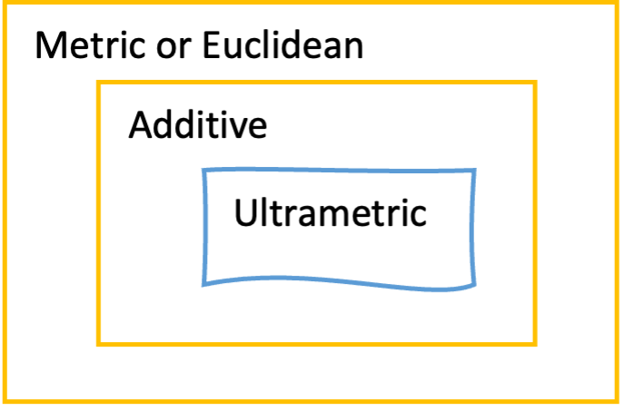
Fig. 3.28 Credits: CC BY-NC 4.0
[Ridder et al., 2024]#

Fig. 3.29 Credits: CC BY-NC 4.0
[Ridder et al., 2024]#
Euclidean or metric distance (Fig. 3.28) requires observed distances to be non-negative, symmetrical, distinct and to obey the triangle inequality (Fig. 3.29, (left): the distance between any pair of sequences a and b cannot exceed the sum of the distances between those sequences and a third sequence c.
Ultrametric distances are characterised by ultrametric inequality (Fig. 3.29, right): the two largest distances, when comparing three sequences, are equal (in this case 6 = 6). Ultrametric distances have the attractive characteristic that they evolve clock-like, and hence that the most similar sequences will also be most closely related. In fact, the ultrametric tree (Fig. 3.27) perfectly describes the observed distances as shown in the distance matrix.
Neighbor Joining#
Probably the most commonly used distance tree building method is Neighbor Joining (NJ), which is fast and effective, especially for large MSAs (with hundreds of sequences). NJ tree building starts with a fully unresolved tree, containing all sequences in an MSA, and calculates a total tree length (or overall starting distance) by summing all pairwise distances. Subsequently, a pair of sequences is chosen and combined to start a small cluster (‘neighbors’) and the total tree length is updated, now replacing the two original by the joined taxa. This step is repeated until all sequences and pairs are joined, whilst minimizing the overall distance (tree length) between them (Fig. 3.30).
Neighbor Joining produces unrooted trees and therefore, if needed, outgroup rooting should be applied in order to root the tree. There is no molecular clock assumption, which allows differences in branch lengths between neighbors (sisters) to be reconstructed. NJ is implemented in MEGA11[Tamura et al., 2021]) and used in the practical.

Fig. 3.30 Neighbor Joining. An illustration of the computational process. Tree length S is the sum of all branch lengths, and is minimized (F) by iteratively joining neighbors, starting from the star tree (A). Credits: CC BY-NC 4.0 [Ridder et al., 2024].#
NJ is highly popular as it can generate trees with hundreds of terminals in a very short time. This makes it a great tool for quickly assessing the (phylogenetic) structure in a data set (MSA) without having to explore wide tree spaces (as in the character-based approach). It is good to keep in mind that NJ is a clustering method, i.e., it groups sequences on the basis of overall similarity, not on shared ancestry or synapomorphy. Therefore, for phylogenetic studies, character-based analysis is preferred, and NJ analysis can be used in addition (Fig. 3.31), to check for possible incongruencies between the two. If these are found, it could mean that the data (the synapomorphies accumulated in the MSA) are not metric for that part of the tree, which could warrant additional analysis methods (such as phylogenetic network reconstruction) which is beyond the scope of this course.
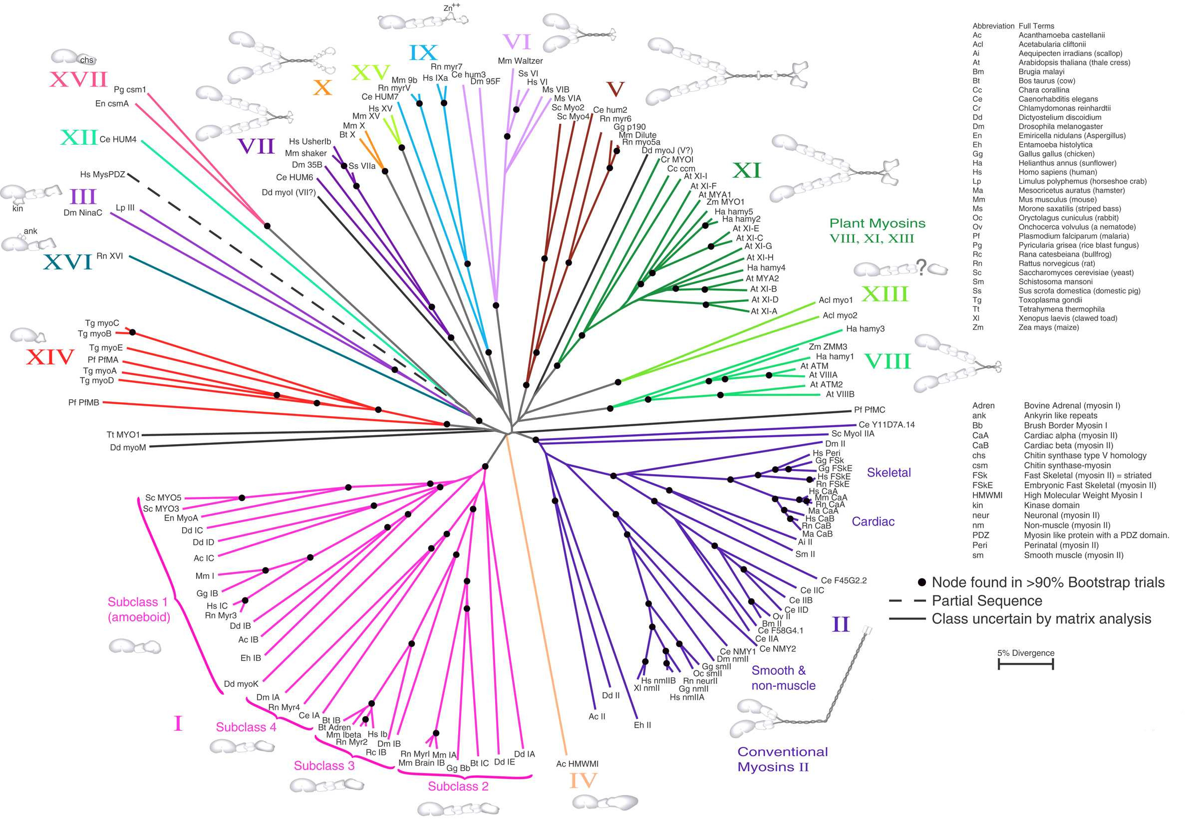
Fig. 3.31 Neighbor Joining. An unrooted NJ tree based on Myosin amino acid sequences. The scale bar indicates 5% sequence divergence. Credits: CC BY 1.0 [Hodge and Cope, 2000].#
Estimating sequence divergence#
In a phylogeny, when there is a combination of long terminal branches combined with short internal ones phylogenetic reconstruction is usually problematic when using nucleotides and parsimony analysis. The reason for this is that on long branches (i.e., with highly-divergent sequences) the chance of any of the 4 nucleotides occurring in both branches at random, is actually quite high and can result in false synapomorphies. After some of these have accumulated, wrong clades can be the result. This so-called long branch attraction (LBA) artefact is fairly common, whenever isolated old lineages (such as Amborella or Nymphaea in the angiosperms) are involved but can also occur in gene trees. LBA has been shown to be mitigated to some extent by modelling branch lengths, rather than merely counting differences as branch length, as in parsimony where each substitution occurring in the MSA results in one extra step of treelength. For the accurate estimation of branch lengths in a phylogenetic tree however we need accurate sequence divergence estimation.
Evolutionary divergence (or distance) between homologous sequences is reflected in substitutions between them since splitting-off from their MRCA. Intuitively, when comparing two sequences, one would just take the proportion of differing sites as sequence divergence, for instance, for a sequence of 1000 positions, having 10 differences would yield 0.01 or 1% difference. However, this so-called p-difference does not necessarily consider all substitutions that historically occurred during divergence of the two sequences (which may include reversals to the original state). Estimating ‘true’ sequence divergence means that we need to find substitutions that did happen but are not visible in your MSA. Variable sites can actually keep on changing during evolution, causing multiple substitutions to occur at the same position, which can lead to saturation of change. In this way several substitutions may go unnoticed, and a mere p-difference will underestimate actual sequence divergence.
Substitution models#
Substitution models, all based on the Jukes-Cantor (JC) formula given below, correct divergence estimates for unobserved events. The JC formula is based on calculation of the chance of having a substitution for a particular site plus the chance of it not changing into any of the three other nucleotides for that site. In the formula, \(p\) stands for the observed proportion of differences (i.e., the p-difference), and \(d\) for the corrected divergence measure. When all sites differ (i.e., \(p = 1\)), \(d\) reaches 0.75 in the limit, i.e., the corrected \(d\) cannot exceed 75%.
Fig. 3.32 shows how the JC formula is applied in a model of substitution, the JC model. There is a matrix defining the six possible substitution types among the 4 nucleotide bases, i.e., T↔C, A↔G, A↔T, T↔G, C↔G, and C↔A. In this case the relative rates for all six substitution types are assumed to be equal and denoted by one shared parameter, named ‘a’. Another assumption in this model is that the base composition across the MSA is equal, assuming a 25% probability of finding of each base at each position in each sequence. The JC model is considered a fairly simple, one parameter, model.

Fig. 3.32 The Jukes Cantor model (left), transitions (blue) and transversions (red) and how they accumulate differently during evolutionary time (right). Credits: CC BY-NC 4.0 [Ridder et al., 2024].#
The first two substitution types listed above are transitions (substitutions among the pyrimidines T and C, and among the purines A and G), whereas the other four occur between purines and pyrimidines and are referred to as transversions. The rate of transitions (ti) has a different dynamic, and hence build-up of substitutions, compared with the rate of transversions (tv) (see Fig. 3.32). In the Kimura 2-parameter (K2P) model (Fig. 3.33) this is accounted for by adding an extra parameter b. Parameter a now estimates ti (\(P\)) and parameter \(b\) estimates tv (\(Q\)); in the Kimura 2 Parameter formula, \(P\) and \(Q\) are the proportions of ti and tv, respectively:

Fig. 3.33 The Kimura 2-parameter substitution
model with transitions indicated in
orange (parameter a) and transversions
in blue (parameter b).
Note that base frequencies fN
are considered equal in this model.
Credits: CC BY-NC 4.0 [Ridder et al., 2024].#
Besides the JC and K2P models, other models exist that take into account different aspects of DNA sequence evolution, such as differences between all six substitution types (general time reversible or GTR), sequence base composition or nucleotide frequencies (Felsenstein81 or F81), and the distribution of rates of change in sites throughout the MSA: how many fast, and how many slow-evolving sites are there and how are they distributed (this is achieved by comparison with a gamma Γ distribution). The most complex models, with many parameters, will consist of combinations of all these aspects of DNA sequence evolution. There are up to 220 different models to choose from. It is good to realise that these models are reversible and therefore allow the reconstruction of unrooted trees only. Once these are determined they can be rooted using outgroup rooting.
For amino acid sequence comparisons, instead of estimating parameter values from the data, amino acid substitution models are based on (pre-defined) substitution cost matrices (see chapter 2) that are based on observations of amino acid substitutions found in over 30,000 protein sequences (e.g., the JTT, Blosum, Dayhoff, LG and WAG matrices).
Maximum likelihood tree building#
For character-based approaches these substitution models, as they are based on probabilities, allow us to calculate the likelihood of our data supporting a particular tree and model. This likelihood is a score describing how well data, tree and model fit together:
Or described in words: the likelihood \(L\) is the probability of obtaining the data \(D\) given hypothesis \(H\), which includes the substitution model and tree selected. We could therefore also say:
Obviously, it is important to select the best fitting model for the data set (MSA). Model selection proceeds by calculating the likelihood for your MSA using a range of different models and the same tree; the best resulting likelihood scores imply the best-fitting model.
Subsequently, a candidate tree is considered and the likelihood LD of observing the data (the MSA) is calculated given that model and that particular tree. Then, another tree is considered whilst the same best-fitting model remains selected, and its parameter values are estimated again. The likelihood LD of observing the data (your MSA) is calculated again and this time the likelihood may actually be better. More trees are evaluated, and more model parameter values are considered, all the time keeping track of LD until no further increase LD can be obtained. This is usually achieved by using the heuristic tree search approaches as outlined in Tree space and heuristic search methods and depending on the tree space, determined by the number of sequences in the MSA. The end result is the maximum likelihood estimate (MLE): the combination of a tree and model parameter values that maximizes the likelihood of the data. This tree, which may not be the exact best MLE (it is after all heuristics), is then usually referred to as the ML tree.
Phylogenetic tree reconstruction based on MLE has become the dominant tree building approach over the past decade. It is an efficient method that can consider differences in substitution rates and patterns between the sequences in an MSA. This would mean that non-clocklike or biased (non-random) accumulation of substitutions would be modelled, and this would minimize possible artefacts in inferring the ML tree topology, for instance LBA (see above).
The MLE pipeline for phylogenetic reconstruction is implemented in the software package IQ-TREE [Minh et al., 2020], which includes I) model testing, II) ML tree search, and III) bootstrapping for both nucleotide and amino acid sequences. IQ-TREE will be demonstrated and used in this chapter’s practical.
Finally, estimating evolutionary divergence using nucleotide substitution models can also be applied in a distance approach. There, the substation models are applied to calculate ‘corrected’ pairwise sequence distances, which are then used to produce a Neighbor Joining tree (see Fig. 3.30)
Model-testing, ML tree search, Bootstrapping#
After an ML tree with branch lengths has been obtained, there is still no information on how nodes in the ML tree may differ in terms of support by the data (MSA). Therefore a bootstrap analysis is carried out, repeating the MLE process a number of times, based on pseudo-replicate data sets drawn from the MSA (see Nodal support in phylogenetic trees: the bootstrap). After an ML tree is obtained for each pseudo-replicate data set, a 50% majority-rule consensus tree is calculated in order to see the group frequencies (the proportion of replicates in which each node is occurring). These frequencies are also referred to as bootstrap values. The idea is that the more synapomorphies a node has, the higher its bootstrap value will be.
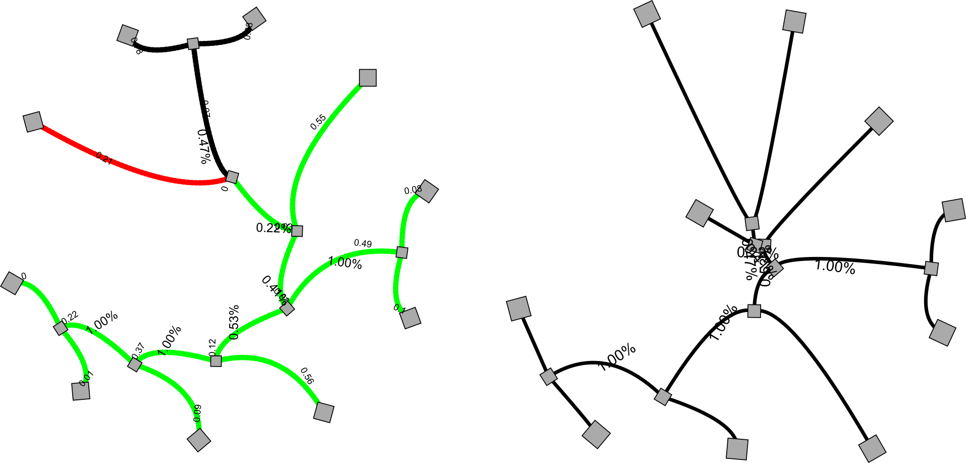
Unfortunately, there is no simple linear relationship between character support and bootstrap values. Generally, bootstrap values < 90% are considered poor support for that node, and values < 50% (or even < 60%) as ‘no support’. Bootstrap values of 62% are usually obtained for MSAs containing one synapomorphy, meaning that such nodes should probably be ignored but this depends on the experience and interpretation of the analyst. Fig. 3.34 illustrates what happens to bootstrap consensus trees when poorly supported nodes are collapsed: the tree topology becomes less well resolved but what is left is strong. That is indeed the trade-off: visualizing lots of nice but poorly supported resolution versus only focusing on strong nodes. Usually, we want to see both.

Fig. 3.34 Bootstrap analysis. A) A maximum likelihood tree with bootstrap values indicated at nodes. Note that not all nodes show a bootstrap value, which is probably because values < 50% are ignored. B) The same analysis, but this time all nodes with bootstrap values < 50% collapsed. Note the introduction of a polytomy containing four lineages resulting from collapsing weak nodes, and the change from additive tree to cladogram style in the collapsed tree. Credits: CC BY-NC 4.0 [Ridder et al., 2024].#
Recap tree building methods#
To summarize, tree building methods can be classified according to the type of data used, characters (or ‘sites’) versus pairwise distance, in which case we also refer to this as clustering analysis. Using characters for tree building results in applying an optimality criterion in order to select among several (sometimes enormous numbers of) candidate trees. Clustering usually results in a single tree, the optimality criterion approach in several, in which case a consensus tree is calculated.
Another useful criterion to classify tree building methods is whether an explicit model of character evolution is applied, versus mere counting (parsimony) of changes. In this course we covered Maximum Likelihood and parsimony, and Neighbor Joining using corrected distances, i.e., applying the character model in pairwise sequence comparison. Bayesian Inference, in which probabilities for nodes are calculated, and different models are evaluated simultaneously, is beyond the scope of this course. (If you are interested, they are covered in BIS-40306 Comparative Biology & Systematics).
Data → |
Distances (pairwise) |
Sites (characters) |
|---|---|---|
Approach ↴ |
||
Explicit model of character evolution |
Neighbor Joining |
Maximum Likelihood |
No model of character evolution |
p-difference |
Parsimony(‘counting’) |
Criterion? |
Clustering |
Optimality criterion |
Glossary#
This glossary contains the most important terms from this chapter.
Glossary
- Apomorphy#
Derived character state
- Autapomorphy#
For a group, all members being derived from one MRCA
- Bifurcating#
A tree containing nodes that are all connected through three branches
- Bootstrap#
A method for measuring node support in a phylogenetic tree
- Branch length#
The length, either in steps (parsimony), distances (clustering) or substitutions per site (maximum likelihood)
- Clade#
Monophyletic group, MRCA with all descendants
- GTR#
General time reversible nucleotide substitution model
- JC#
Jukes-Cantor nucleotide substitution model
- K2P#
Kimura 2-parameter nucleotide substitution model
- LBA#
long-branch attraction
- Monophyly#
For a group, all members being derived from one MRCA
- MLE#
Maximum likelihood estimate
- MRCA#
Most recent common ancestor
- MSA#
Multiple sequence alignment
- Nodal support#
The support -by the characters- for a node in the phylogenetic tree
- Paraphyly#
For a group, not all members being derived from one MRCA
- p-difference#
Proportional difference, uncorrected
- Polytomy#
Part of a phylogenetic tree that is collapsed, node is connected through > 3 branches
- Root#
Reference individual, used for polarising a tree
- Synapomorphy#
Shared derived character state
- Transition#
a substitution among pyrimindes (C,T) or among purines (A,G)
- Transversion#
a pyrimidine ↔ purine substitution
Practical assignments#
This guide contains questions and exercises to help you process the study materials of Chapter 3. You have two mornings to work your way through the exercises. In a single session you should aim to get about halfway through this guide, i.e., assignments I-IV. Note that assignment VI is optional.
These practical exercises offer you the best preparation for the project in Week 6 and the tools and their use are also part of the exam material. Thus, make sure that you develop your practical skills now, in order to apply them during the project and to demonstrate your observation and interpretation skills during the exam.
Note, the answers will be published after the practical!
Assignment I: Make an amino acid based PLT1 tree in MEGA11 & visualize it in iTOL (30 minutes)
As a start, in this assignment you are going to express relationships among a set of 10 PLT1 amino acid sequences for which you generated a multiple sequence alignment (MSA) last chapter. You will do this by building a parsimony tree, using Molecular Evolutionary Genetics Analysis (MEGA 11). You will then visualize your tree using the tree figure software FigTree and using iTOL, which is a highly useful platform for storing, managing trees and making pretty pictures of them.
First, Start MEGA 11 and open and have a look at the standard MEGA 11 dashboard available to you. The open white field works as a canvas on which each analysis performed will appear as a pinned note. Apart from ‘PHYLOGENY’ there are many interesting tools available, some of which you will be using today.
Using File > Open, open your PLT1 MSA from last chapter; this file should be a FASTA file, with the extension .fasta in the file name.
When presented with a choice between Analyze and Align, select Analyze (as the sequences are aligned already).
Next, select the correct data type.
Have a look at your alignment by selecting
Data > Explore Active Data(or hit theTAbutton), which will bring you into the DataExplorer.Using the settings
Display > Color Cellsyou can see clearly how the amino acids align, and how stretches of high conservation alternate with highly-variable parts of the alignment.Clicking the
TAbutton enables you to highlight non-identical amino acids per alignment position, which can be useful especially in big alignments of 100+ sequences.
Now close the Data Explorer which will return you to the MEGA dashboard and click Phylogeny > Construct/Test Maximum Parsimony Tree(s).
Leave the default setting, which includes ‘no test of phylogeny’ (bootstrapping) and ‘MP search Method’ is the SPR branch swap.
Confirm and use default settings for computing the tree;
After a few seconds you will see your tree, which is in cladogram style (there is no branch length information, it is topology-only).
In order to see the branch lengths, select ‘Layout’ (in the top-left window) and then Toggle scaling of the Tree which calculates branch lengths for this tree; this should take <2 minutes.
Select ‘Branch lengths’ and you see the average number of amino acid replacements indicated on the branches of the tree (average across multiple possible optimizations for each position).
One good thing of MEGA is that upon clicking Caption (bottom left) you will get complete info on all the settings that were used in this analysis as well as on results; for instance, how many most parsimonious reconstructions there were (in this case a single one), how starting trees were calculated and how many sites were in the MSA.
Now save your tree by selecting
File > Export Current Tree(Newick), tick the ‘Branch length’ box, and click ‘Ok’. The Newick notation will be shown in the Text File editor, selectFile > Save asand give it a logical name and replace the .nwk extension by .tre.You may repeat the Maximum parsimony analysis, but now selecting, at ‘Phylogeny Test’,
Bootstrap method. This will perform a bootstrap analysis of 500 replicates.After it is completed you see two tabs on top of the tree window: ‘Original Tree’ shows the initial parsimony result now with bootstrap values superimposed on (some of) the nodes. The other tab, named ‘Bootstrap consensus tree’ shows the actual bootstrap analysis.
Use Layout >
Toggle scaling of the treein order to see the average branch lengths.Save your bootstrap tree as above, now with ticking the
Bootstrap Valuesbox.
We have seen in the lectures that boostrap values of < 50% are actually rather uninformative, as a single synapomorphy already can have 62% as a result. Therefore, it will be good to take a look at the ‘condensed’ version of our tree.
Make sure you are in the Original tree tab and go to
Compute > Compute condensed treebutton (top-left). You will be given ‘Tree Cutoff options’ and type 62 in the % cutoff box. See how your tree changes?
Questions:
Why are the topologies of the bootstrap consensus and that of the most parsimonious tree not the same?
What does the polytomy in your condensed tree represent?
Visualising your trees is an essential step in phylogenetic analysis, as the (hierarchical) information contained in trees is usually graphical in nature. Important aspects of picturing phylogenetic trees are:
Tree structure: most clearly visualized in the rectangular-style version of your tree, but with larger number of taxa (terminals) the tree won’t fit on one page anymore and a circle tree (cladogram style) may be a better solution.
Branch lengths; the amount of evolution that occurred across your taxa or genes and therefore of interest in itself; again, with large numbers of terminals, a circle tree (with additive branch lengths) is probably a better solution.
Nodal support: usually bootstrap values (group frequencies) are depicted, but these can also be indicated by symbols or by proportional widths of branches subtending that node; see below.
Rooting: the effect of outgroup-rooting should be clearly visualized.
FigTree A stable and practical tree visualisation tool, which is fully freeware, is FigTree which can be obtained from here. A video is included on Brightspace outlining how to use FigTree for a nice visualization of a tree with bootstrap values attached, see tomorrow’s IQ-TREE practical.
iTOL The iTOL platform provides quite useful solutions to accommodate all these aspects in your tree picture. We will run through some of them here. Most of iTOL’s functions are free, but for saving results and treeviews a subscription is required.
For now, go to iTOL and register for getting a (free) account there. At the Welcome page, do have a look around to get a feel for how larger trees can be displayed and additional (external) data can be integrated and annotated with the tree figures. Also, do have a look at the Gallery where user trees are displayed.
Go to MyTrees and upload the two trees that you just made in MEGA 11.
Clicking on either of them will visualize your trees.
N.B.: the Control panel can be dragged to the side in order to see the entire tree. Use the previous and next tree buttons (next to My Trees) in order to toggle between the two trees.
Although no outgroup was included or selected in your PLT1 MSA, the tree appears rooted because in the Control Panel under Mode ‘Rectangular’ is selected by default in iTOL.
Therefore, you want to show the tree unrooted by selecting ‘Unrooted’.
Under
Branch options > Line styleincrease the line thickness to up to for instance 20 px in order to make the tree structure more clearly visible.Under
Labelstoggle between Display and Hide in order to see tree structure-only; use the + tool (top-right corner of the screen) to zoom in.Under
Mode options > Rotationyou can rotate your tree.Now make sure to select your bootstrap consensus tree and go to
Advanced > Branch metadata > Display > Bootstraps / metadataand select ‘Display’ and then ‘Text’. Increase font size to like 60px, Round to 2 decimals and you see your bootstrap values appear at your tree.Go to
Advanced > Node optionsand select ‘Display’ for both your Leaf nodes and Internal nodes. Choose a symbol and colour, increase the symbol size to like 50px or more.Now switch to your ‘Original tree’ and use
Advanced > Branch metadata display > Branch lengthsand select ‘Display’. Increase font size to like 60px and Round decimals to 2; this way you can read your branch lengths from your tree.Go back to
Basic, make sure ‘Mode’ is either Circular or Rectangular (not Unrooted) and then selectBranch options > Connections between nodes are curves.Go to
Basic > Mode optionsand select ‘Ignore’ at branch lengths in order to see a cladogram version of your tree, i.e., without proportional branch lengths. N.B.: this will not work for your bootstrap consensus tree as it has no branch lengths. (trees with branch lengths are much more interesting!)Click on any internal node in your tree and select
Branches > This node > Colourin order to colour a branch in your tree.Explore the other functions of tree visualisation that iTOL offers; when you are happy with your tree, use
Export > Full image > Exportand save in .svg format, for use in Word or PowerPoint documents.
Switching the terminal labels back on (using Basic > Labels > Display) it is clear that for this picture the sequence names are too long. This is best edited manually in the .fasta file you started with.
Last but not least: placing a root on your tree, in case you do have outgroup information, is possible by selecting a node or branch (can be internal and terminal ones) and selecting
Editing > Tree structure > Re-root the tree here. In case you would want to re-root again you need to Reset the tree first (in Control panel the yellow button bottom-right).
With these steps you have gone from a tree generated in MEGA 11 to a nice tree picture, a procedure that you can apply to other trees generated in this practical and of course in your project later on in the course. Also, use iTOL to store your trees and keep an overview of all trees generated.
Assignment I answers
Why are the topologies of the bootstrap consensus and that of the most parsimonious tree not the same?
Probably because they are un-rooted or rooted differently. In case an outgroup is known, rooting it with that would probably give it same or at least congruent topologies. Alternatively, when rooted properly, it could still be that some weak nodes in the parsimony tree didn’ t make it in the bootstrap consensus. This would also cause topology changes, though not necessarily incongruence.What does the polytomy in your condensed bootstrap tree represent?
That there not enough synapomorphies in the MSA to resolve the -now collapsed- nodes in the polytomy. Alternatively, it could also bet he cases that there are enough, but conflicting, synapomorphies. That way you would also get a polytomy.
Assignment II: Estimating sequence divergence: exploring the MSA (20 minutes)
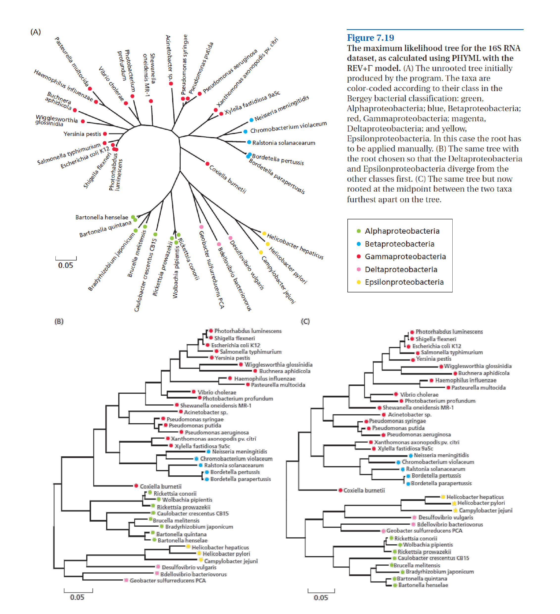
Proteobacterial 16S rDNA sequences (see above; from [Zvelebil and Baum, 2007]) have been compiled and aligned for 38 species of bacteria from the phylum Proteobacteria, which is usually divided into five classes: α-, β-, γ-, δ-, and ε-Proteobacteria (see here for further background for this phylum). The 38 species included here are spread across these five classes, therefore phylogenetic reconstruction should be able to recover five clades, if this classification is indeed based on evolution. In this practical you will estimate sequence divergence and then phylogenetic relationships among these 38 rDNA sequences.
First you are going to explore divergence in a multiple sequence alignment (MSA), and how to make corrections to the crude, proportional p-differences between sequences, in order to estimate their ‘true’ evolutionary divergence.
Start MEGA 11 and open the 16S rDNA sequence alignment provided on BrightSpace (by selecting Data > Open A File/Session) and select Analyze.
Then select the appropriate data type, keeping in mind that 16S rDNA is not protein coding sequence.
Now explore the SSU sequence alignment using the DataExplorer (Data > Explore Active Data).
Using the settings Display > Color Cells you can see clearly how the nucleotides align, and how stretches of high conservation alternate with highly-variable parts of the alignment.
(This is relevant later on for choosing the right nucleotide substitution model when calculating a likelihood tree).
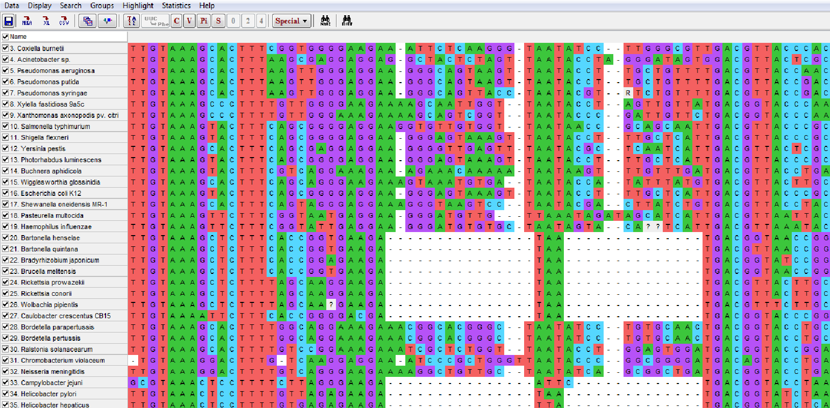
The C, V, Pi and S buttons at the top allow you to highlight specific sites according to conservation, variability, phylogenetic (‘parsimony’) information or single changes, i.e., occurring in just one sequence.
Parsimony informative (Pi) sites have a nucleotide different from the rest in at least two sequences.
Such sites have the potential to build at least the smallest clade possible, that of two terminals.
Counts for each category are given in the lower left corner of your screen.
Clicking the TA and C buttons, enables you to highlight conserved sites throughout the alignment.
You will see that there are some gaps in the alignment where only one or a few sequences are present. This alignment does not contain an outgroup sequence, therefore, in principle, we can only produce unrooted trees later on.
Questions:
What do the alignment-gaps represent?
What is the % of phylogenetic informative (Pi) sites in this alignment?
How could we try and find a proper outgroup sequence for our alignment?
Given that our trees will be unrooted can we still infer monophyly of the different Proteobacterial classes?
Assignment II answers
They represent length-variation among the sequences (not ‘holes’ in the DNA…) and have been decided by the operator compiling the alignment, i.e., there can be subjectivity in where exactly to place the gaps.
These can be found in the bottom–left window corner: V=828, Pi=666, both out of 2444 total sites (34% and 27%) Pi sites are sites in which at least two sequences have a nucleotide different from the rest. Such sites have the potential to build at least the smallest clade possible, that of two terminals.
When we know that an outgroup has not been included in our ingroup (i.e., the set of sequences the phylogenetic relationships among which we want to estimate) an additional sequence, probably from GenBank or other data bases, would need to be added. BLAST or psiBLAST might be a good tool to find sequences that share an MRCA with our ingroup, by selecting among BLAST hits those sequences with a sequence divergence greater than that among ingroup sequences. (But be aware that these could also represent ‘outcast’ sequences rather than outgoups!) Alternatively, the (taxonomic) literature may be useful to guide outgroup selection.
No, strictly speaking not (“no rooting no monophyly…”). We would need that outgroup! On the other hand, it is tempting to consider the main ‘clades’ in your tree as clades indeed, especially when the MRCAs for each are on long branches apart from each other. Wilkinson et al. have suggested to call these ‘clans’ instead of ‘clades’. Possibly, the different clades may not change so much upon different rooting scenarios. Their relative branching order may well do.
Assignment III: Estimating sequence divergence: Pairwise distances (30 minutes)
Now close the Data Explorer and go to Distance, for computing a pairwise distance comparison among all sequences in the alignment.
Select Compute Pairwise Distances.
First you will make a crude, uncorrected, distance measure by selecting p-difference, which is basically the proportion of differing sites between any two sequences (like the %-identity score you have seen in chapter 2).
Click in the areas in the Setting part (next to the Option part) of the Analysis Preferences window and use the following settings:
Variance estimation Method = None.
Model/Method = p-distance.
Substitutions to include = Transitions + Transversions.
Rates among sites = Uniform rates.
Gaps/Missing Data Treatment = Pairwise deletion.
and click Ok.
From the Average menu, select Overall.
What is the overall average sequence divergence among these sequences?
Now repeat the above steps but this time selecting Kimura 2 parameter (K2P) model.
What is now the overall average distance?
(Always use the Caption menu option to verify what your settings were).
We have seen in the Data Explorer that there are highly conserved but also highly variable sites in our alignment.
Assuming Uniform rates among sites may therefore not be realistic.
Repeat the above steps again, this time selecting both K2P model and Rates among sites = Gamma distributed (G).
What is now the overall average distance?
Actually, we would also like the base composition in our sequences to be able to differ from the 1:1:1:1 which was so far assumed.
Therefore, keeping all other settings equal to your settings as before, now select the Tamura-Nei (TN) model under Model/Method and calculate your overall average distance.
Finally, you will recall there were some large gaps in the alignment.
Therefore, repeat the last step but this time changing Gaps/Missing Data Treatment to Complete deletion.
What is the overall average distance now?
Questions:
Why do these distances values get increasingly larger (apart from the last step)?
Can you think of cases where the raw p-difference would be ok for measuring evolutionary distance?
What is Complete deletion (check your Captions) and how does it compare with Pairwise deletion?
In your opinion, what would be the best way of modelling sequence divergence among these sequences?
Assignment III answers
From the Average menu, select Overall. What is the overall average sequence divergence among these sequences?
0.183.
Now repeat the above steps but this time selecting Kimura 2 parameter (K2P) model. What is now the overall average distance? (Always use the Caption menu option to verify what your settings were)
0.213.
Repeat the above steps again, this time selecting both K2P model and Rates among sites = Gamma distributed (G). What is now the overall average distance?
0.25.
Now select the Tamura-Nei (TN) model under Model/Method and calculate your overall average distance.
0.253.
Repeat the last step but this time changing Gaps/Missing Data Treatment to Complete deletion. What is the overall average distance now?
0.227.
It is because increasingly more realistic/sophisticated modelling of sequence divergence is taking into account increasingly more ‘unseen events’. Simple models such as Jukes-Cantor can’t notice the subtleties that the more expensive models can.
In case of recent divergence where only few substitutions have ocurred. For instance, among DNA barcodes for species ID.
Sequences are being compared on a pair-wise basis, i.e., everybody is compared with everybody. When there is length-variation present in the MSA, comparison of positions lacking in one sequence cannot be made. Such positions could then be ignored for that comparison (between those two sequences) and this is Pairwise deletion. The alternative can be Complete deletion in which the entire columns (positions, characters) in which this length-variation occurs is deleted prior to pairwise comparison. This way you end-up with an MSA in which no length-variation exists anymore and quite possibly, in the process you will have ‘thrown away’ some valuable variation (substitutions) in the length-variable regions. Especially if the length variation contained long indels.
Ideally this would depend on the overall level of sequence similarity, or p-distance: if it is < 2% use JC or K2P, if it is > 5% use GTR and if you see high-diverse regions alternated with ‘quiet’ ones definitively use Gamma! The idea is that the higher the p-distance the more evolution has occurred and probably more sophisticated models are needed to describe all that. In this case p-distance was 0.183 which is already pretty high. Therefore, a more complex (‘expensive’) model is better here. The other thing is that because of some very large inserts the complete deletion option may be better(?), although for smaller gaps and inserts (‘indels’) this means sacrificing a lot of variation (synapomorphies!). Best to try both complete and pairwise deletion and assess and discuss difference in results, if any.
Assignment IV: From sequence divergence to trees: Distance trees (60 minutes)
After having computed Pairwise Distances among the sequences, you will now perform distance tree analysis (NJ), converting pairwise sequence distances into (distance) trees.
Using MEGA 11, under the Phylogeny menu construct two Neigbor Joining trees: one based on p-difference and use Uniform rates (for ‘Rates among Sites’), Complete deletion (for ‘Gaps/Missing Data Treatment’) and one based on what you consider the best model/treatment given your answer to assignment III, question 4 above, including ‘Gamma Distributed’ rates.
Can you see a difference in (tree) result?
Now repeat the best model+Gamma analysis, this time using Pairwise deletion (instead of Complete deletion).
There should be a Heliobacter/Campylobacter + Desulfo/Geobacter Bdellovibrio clade.
You can root with this clade by I) clicking its stem-branch, and II) use Subtree > Root tree.
Check how your tree topology may have changed now.
On the same tree, in the Tree Explorer now use the Options button (at the top of the window, left from the i button) to display the tree formatting tools, used to make your two trees look pretty.
(You can also use TaxonNames > ShowTaxonMarkers > Markers).
Use the Tree, Branch and Labels tabs and explore the various options.
For instance, change the appearance of your tree, switch branch lengths on/off as you prefer and use the Labels tab to mark the α, β, γ, δ, and ε Proteobacteria with their own colour and shape (for an example, see the figure in assignment II, above).
Save an image of your tree using Image > Save as PNG file.
Remember this analysis is actually unrooted, therefore also produce an unrooted visualisation of your trees by selecting Radiation from View > Tree/Branch Style.
This is exactly the same tree structure with the same branch lengths, but it is not ‘polarised’ and therefore the existence of clades in it dependent on root-choice.

Questions:
Keeping in mind the dependence on root-choice, what can you say about monophyly of the α-, β-, γ-, δ-, and ε- Proteobacteria based on this sequence alignment?
Applying the rooting as above (assigning Bdellovibrio and Heliobacter as outgroup, are your NJ trees congruent with those depicted in that figure? If not, what could be the cause?
Assignment IV answers
With Neighbor Joining, using Tajima Nei substitution model and with gamma modelled rate distribution (shape parameter α=1), there is monophyly of the beta class (blue), for the gammas (red) their MRCA would also have lead to the beta class, therefore the gammas are paraphyletic. The other three classes are each monophyletic, however this may change when proper rooting is applied.
Below is the same NJ tree as in step 1 above, left: rooted on delta+epsilon , and right: mid point rooted (both trees based on Pairwise deletion). This result in a different placement of the α class (green, which is sister to yellow and purple in the mid-point rooted tree), but as the internodes connecting this clade are very short (i.e. not many characters supporting it), this topological incongruence is weak and therefore we don’t attach main conclusions to it.
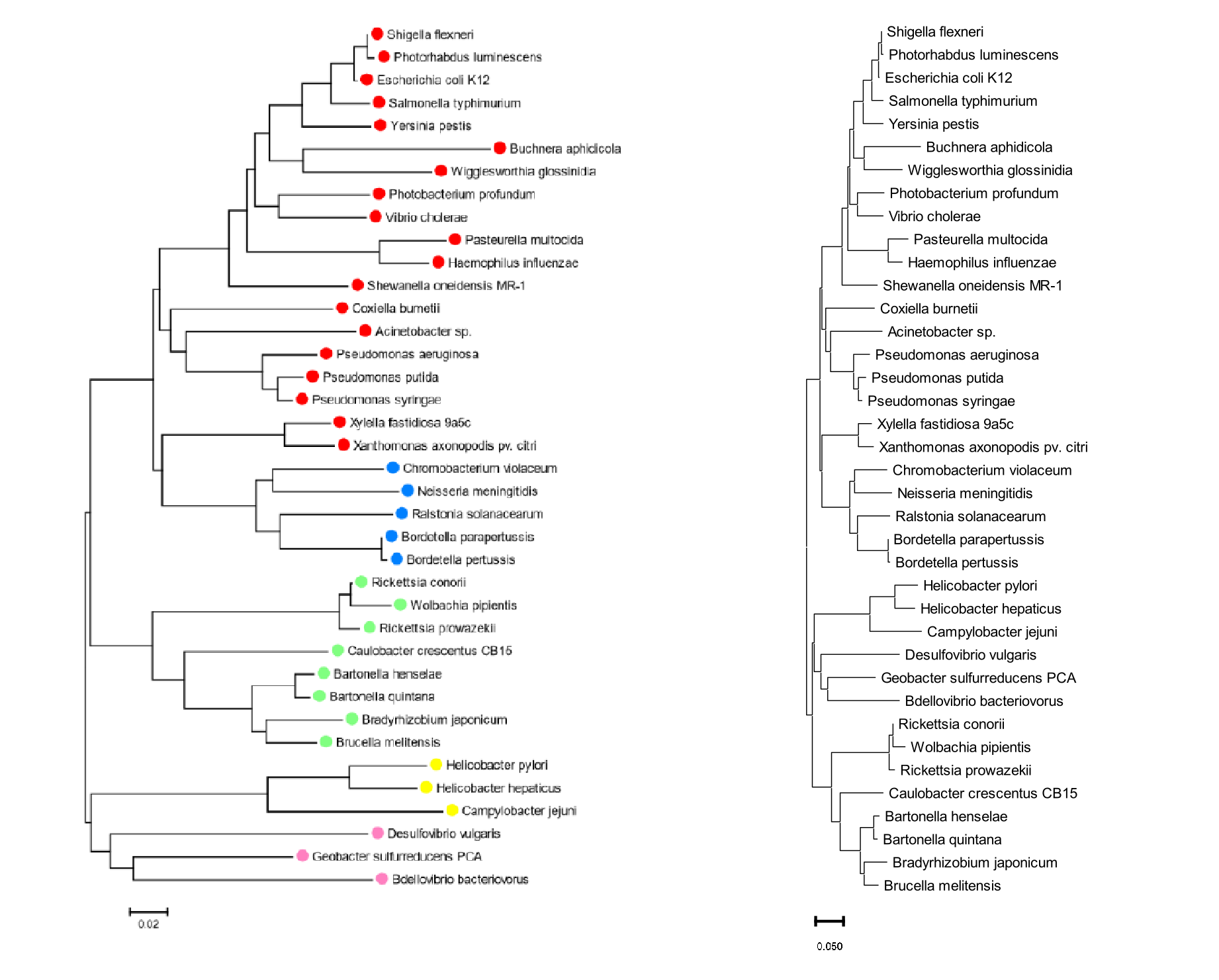
The only difference with the trees from assignment II (from Zvelebil & Baum) is with regards the placement of Coxiella burnetii, which is nested in the red cluster in our NJ trees, but sister to red+blue in Zv&B. The trees seem different with regards to the placement of yellow, green and purple, but all trees, ours and Zv&B have ((yellow, purple)green), it’s just that in Zv&B this clade is flipped/turned around. This does not affect the information in the tree (which is hierarchical) and therefore there is no conflict among the trees with regards this part.
The reason for the different placement of Coxiella burnetii could well be the fact that in Zv&B maximum likelihood was used whereas our trees are NJ distance trees.
Assignment V: From sequence divergence to trees: Likelihood trees (60 minutes)
With the maximum likelihood (ML) approach an explicit model of nucleotide substitution is applied in order to calculate the probability of ‘observing the data’. This means that the probability of having each site change as observed is calculated given a certain tree topology (out of many such topologies). Branch lengths on ML trees are rates, expressed as nucleotide substitutions per site.
You will first calculate an ML tree using MEGA and compare this to a commonly used online tool, IQ-TREE.
In MEGA use the Phylogeny button to select Construct/test Maximum Likelihood Tree and compute a tree using the following settings:
Test of Phylogeny = None.
Model/Method = General Time Reversible model.
Rates among Sites = Gamma Distributed (G).
Gaps/Missing Data Treatment = Complete deletion.
ML heuristic method = SPR level 5.
Initial tree for ML = NeighborJoining.
Branch swap filter = None.
ML heuristic method: a branch swapper used to ‘jump’ from tree to tree during the ML search; ‘Initial tree for ML’: the starting tree for this search.
After the analysis has finished (usually a few minutes) male your ML tree look pretty and produce an unrooted version (as you did before), and check the Caption for the log likelihood value obtained for this analysis. You may want to de-select ‘Branch Lengths’. How do the five Proteobacterial classes group in this analysis? Is the ML tree topology different from the NJ tree you calculated under at the start of assignment IV?
For comparison, now go to IQ-TREE where you will see three modules:
‘Tree Inference’, ‘Model Selection’ and ‘Analysis Result’. Select ‘Tree Inference’ and simply upload your original Proteobacterial SSU sequence alignment FASTA file and for now just use default options, i.e., do not change anything further.
IQ-TREE is most likely the best and most powerful tool currently around for calculating ML phylogenetic trees, and their associated bootstrap analyses. In case of delays, or when the analysis is taking too long, you can also use IQ-TREE webserver and select Vienna and/or Los Alamos of the 3 Web servers listed there at the top of the page (CIPRES is a pay-site).
Depending on the server load (see top left corner), after an amazingly short time (minutes?) check your status in Analysis Results > Run Log, and keep re-freshing your screen.
When your analysis is finished, proceed straight away to DOWNLOAD SELECTED JOBS button at the bottom-left, and extract the resulting .zip in your own space.
At the Summary tab you can already see your tree result with on the nodes the actual bootstrap support values indicated. At the Analysis Result tab you can see something like this:
ModelFinder
-----------

Best-fit model according to BIC: TN+I+G4

List of models sorted by BIC scores:

Model		  LogL		AIC	 w-AIC	  AICc	     w-AICc   BIC	w-BIC

TN+I+G4		-19303.1910 38766.3819 + 0.0989 38771.8665 + 0.1070 39230.4932 + 0.6952
TIM3+I+G4	-19300.2294 38762.4589 + 0.7035 38768.0829 + 0.7096 39232.3716 + 0.2718
TIM2+I+G4	-19303.0277 38768.0554 + 0.0429 38773.6795 + 0.0432 39237.9681 - 0.0166
TIM+I+G4	-19303.2163 38768.4327 - 0.0355 38774.0567 - 0.0358 39238.3454 - 0.0137
HKY+I+G4	-19313.5323 38785.0647 - 0.0000 38790.4115 - 0.0000 39243.3746 - 0.0011
TPM3+I+G4	-19310.1240 38780.2479 - 0.0001 38785.7325 - 0.0001 39244.3592 - 0.0007
TPM3u+I+G4	-19310.1375 38780.2751 - 0.0001 38785.7596 - 0.0001 39244.3864 - 0.0007
GTR+I+G4	-19300.0064 38766.0128 + 0.1190 38771.9213 + 0.1041 39247.5283 - 0.0001
TPM2u+I+G4	-19313.1016 38786.2031 - 0.0000 38791.6877 - 0.0000 39250.3144 - 0.0000
TPM2+I+G4	-19313.1024 38786.2047 - 0.0000 38791.6893 - 0.0000 39250.3160 - 0.0000
K3Pu+I+G4	-19313.5302 38787.0604 - 0.0000 38792.5450 - 0.0000 39251.1717 - 0.0000
TVM+I+G4	-19309.6489 38783.2978 - 0.0000 38789.0631 - 0.0000 39259.0119 - 0.0000
TIM3e+I+G4	-19325.6629 38807.3257 - 0.0000 38812.5367 - 0.0000 39259.8342 - 0.0000
K2P+I+G4	-19337.4464 38826.8928 - 0.0000 38831.8374 - 0.0000 39267.7985 - 0.0000
TVMe+I+G4	-19326.3815 38810.7629 - 0.0000 38816.1098 - 0.0000 39269.0728 - 0.0000
TNe+I+G4	-19335.6477 38825.2955 - 0.0000 38830.3724 - 0.0000 39272.0026 - 0.0000
SYM+I+G4	-19324.7959 38809.5918 - 0.0000 38815.0763 - 0.0000 39273.7031 - 0.0000
K3P+I+G4	-19337.2939 38828.5878 - 0.0000 38833.6647 - 0.0000 39275.2949 - 0.0000
TIM2e+I+G4	-19334.8067 38825.6134 - 0.0000 38830.8244 - 0.0000 39278.1219 - 0.0000
TIMe+I+G4	-19335.4997 38826.9994 - 0.0000 38832.2104 - 0.0000 39279.5080 - 0.0000
TIM3+G4		-19388.3100 38936.6199 - 0.0000 38942.1045 - 0.0000 39400.7312 - 0.0000
TN+G4		-19395.0111 38948.0221 - 0.0000 38953.3690 - 0.0000 39406.3321 - 0.0000
TIM+G4		-19395.0060 38950.0120 - 0.0000 38955.4965 - 0.0000 39414.1233 - 0.0000
TIM2+G4		-19395.0579 38950.1158 - 0.0000 38955.6003 - 0.0000 39414.2271 - 0.0000
TPM3u+G4	-19398.9953 38955.9906 - 0.0000 38961.3375 - 0.0000 39414.3005 - 0.0000
TPM3+G4		-19398.9978 38955.9955 - 0.0000 38961.3424 - 0.0000 39414.3054 - 0.0000
GTR+G4		-19388.2773 38940.5545 - 0.0000 38946.3199 - 0.0000 39416.2686 - 0.0000
HKY+G4		-19406.5984 38969.1969 - 0.0000 38974.4078 - 0.0000 39421.7054 - 0.0000
TIM3e+G4	-19410.6682 38975.3364 - 0.0000 38980.4133 - 0.0000 39422.0435 - 0.0000
K3Pu+G4		-19406.5536 38971.1072 - 0.0000 38976.4540 - 0.0000 39429.4171 - 0.0000
TPM2+G4		-19406.6104 38971.2208 - 0.0000 38976.5677 - 0.0000 39429.5307 - 0.0000
TPM2u+G4	-19406.6129 38971.2257 - 0.0000 38976.5726 - 0.0000 39429.5356 - 0.0000
TVM+G4		-19398.9225 38959.8449 - 0.0000 38965.4690 - 0.0000 39429.7576 - 0.0000
TVMe+G4		-19410.8116 38977.6231 - 0.0000 38982.8341 - 0.0000 39430.1316 - 0.0000
SYM+G4		-19409.2324 38976.4648 - 0.0000 38981.8116 - 0.0000 39434.7747 - 0.0000
K2P+G4		-19426.4007 39002.8014 - 0.0000 39007.6156 - 0.0000 39437.9057 - 0.0000
TNe+G4		-19424.5670 39001.1341 - 0.0000 39006.0787 - 0.0000 39442.0398 - 0.0000
K3P+G4		-19426.1739 39004.3477 - 0.0000 39009.2924 - 0.0000 39445.2535 - 0.0000
TIM2e+G4	-19423.1694 39000.3388 - 0.0000 39005.4157 - 0.0000 39447.0459 - 0.0000
TIMe+G4		-19424.3389 39002.6778 - 0.0000 39007.7547 - 0.0000 39449.3849 - 0.0000
F81+I+G4	-19618.8625 39393.7250 - 0.0000 39398.9360 - 0.0000 39846.2335 - 0.0000
JC+I+G4		-19637.5080 39425.0160 - 0.0000 39429.8302 - 0.0000 39860.1204 - 0.0000
F81+G4		-19698.1550 39550.3100 - 0.0000 39555.3870 - 0.0000 39997.0172 - 0.0000
JC+G4		-19714.7715 39577.5431 - 0.0000 39582.2286 - 0.0000 40006.8460 - 0.0000
TIM3+I		-19908.5538 39977.1075 - 0.0000 39982.5921 - 0.0000 40441.2188 - 0.0000
TN+I		-19916.7406 39991.4811 - 0.0000 39996.8280 - 0.0000 40449.7911 - 0.0000
TPM3+I		-19919.2576 39996.5153 - 0.0000 40001.8622 - 0.0000 40454.8252 - 0.0000
TPM3u+I		-19919.2588 39996.5177 - 0.0000 40001.8646 - 0.0000 40454.8276 - 0.0000
GTR+I		-19907.7513 39979.5025 - 0.0000 39985.2679 - 0.0000 40455.2166 - 0.0000
TIM2+I		-19915.9636 39991.9271 - 0.0000 39997.4117 - 0.0000 40456.0384 - 0.0000
TIM+I		-19916.6179 39993.2358 - 0.0000 39998.7204 - 0.0000 40457.3471 - 0.0000
HKY+I		-19927.0476 40010.0952 - 0.0000 40015.3062 - 0.0000 40462.6038 - 0.0000
TIM3e+I		-19932.9535 40019.9069 - 0.0000 40024.9839 - 0.0000 40466.6141 - 0.0000
TVM+I		-19917.8824 39997.7649 - 0.0000 40003.3889 - 0.0000 40467.6776 - 0.0000
TPM2+I		-19925.7042 40009.4084 - 0.0000 40014.7553 - 0.0000 40467.7183 - 0.0000
TPM2u+I		-19925.7069 40009.4139 - 0.0000 40014.7607 - 0.0000 40467.7238 - 0.0000
K3Pu+I		-19926.9125 40011.8250 - 0.0000 40017.1719 - 0.0000 40470.1349 - 0.0000
TVMe+I		-19936.2200 40028.4401 - 0.0000 40033.6511 - 0.0000 40480.9486 - 0.0000
SYM+I		-19932.9153 40023.8306 - 0.0000 40029.1775 - 0.0000 40482.1405 - 0.0000
K2P+I		-19948.9891 40047.9782 - 0.0000 40052.7924 - 0.0000 40483.0826 - 0.0000
TNe+I		-19945.7611 40043.5223 - 0.0000 40048.4669 - 0.0000 40484.4280 - 0.0000
K3P+I		-19948.6125 40049.2250 - 0.0000 40054.1697 - 0.0000 40490.1308 - 0.0000
TIMe+I		-19945.4002 40044.8003 - 0.0000 40049.8772 - 0.0000 40491.5074 - 0.0000
TIM2e+I		-19945.7324 40045.4647 - 0.0000 40050.5417 - 0.0000 40492.1719 - 0.0000
F81+I		-20192.9782 40539.9564 - 0.0000 40545.0334 - 0.0000 40986.6636 - 0.0000
JC+I		-20210.8831 40569.7662 - 0.0000 40574.4517 - 0.0000 40999.0692 - 0.0000
TIM3		-21665.4201 43488.8402 - 0.0000 43494.1871 - 0.0000 43947.1502 - 0.0000
GTR		-21659.1410 43480.2820 - 0.0000 43485.9060 - 0.0000 43950.1947 - 0.0000
TIM2		-21674.8531 43507.7061 - 0.0000 43513.0530 - 0.0000 43966.0161 - 0.0000
TN		-21681.2126 43518.4252 - 0.0000 43523.6362 - 0.0000 43970.9338 - 0.0000
TIM		-21680.8091 43519.6182 - 0.0000 43524.9650 - 0.0000 43977.9281 - 0.0000
TIM3e		-21698.1581 43548.3162 - 0.0000 43553.2608 - 0.0000 43989.2219 - 0.0000
SYM		-21691.7915 43539.5830 - 0.0000 43544.7940 - 0.0000 43992.0915 - 0.0000
TIM2e		-21708.9773 43569.9545 - 0.0000 43574.8992 - 0.0000 44010.8602 - 0.0000
TNe		-21715.4418 43580.8835 - 0.0000 43585.6977 - 0.0000 44015.9879 - 0.0000
TVMe		-21710.3436 43574.6872 - 0.0000 43579.7642 - 0.0000 44021.3944 - 0.0000
TIMe		-21714.9849 43581.9698 - 0.0000 43586.9145 - 0.0000 44022.8756 - 0.0000
TPM3u		-21710.9978 43577.9956 - 0.0000 43583.2066 - 0.0000 44030.5041 - 0.0000
TPM3		-21710.9986 43577.9972 - 0.0000 43583.2082 - 0.0000 44030.5057 - 0.0000
TVM		-21705.8439 43571.6879 - 0.0000 43577.1724 - 0.0000 44035.7992 - 0.0000
K2P		-21733.7440 43615.4880 - 0.0000 43620.1735 - 0.0000 44044.7909 - 0.0000
TPM2u		-21719.4587 43594.9174 - 0.0000 43600.1284 - 0.0000 44047.4259 - 0.0000
TPM2		-21719.4609 43594.9218 - 0.0000 43600.1328 - 0.0000 44047.4303 - 0.0000
HKY		-21724.8089 43603.6177 - 0.0000 43608.6946 - 0.0000 44050.3248 - 0.0000
K3P		-21733.2531 43616.5062 - 0.0000 43621.3204 - 0.0000 44051.6106 - 0.0000
K3Pu		-21724.3838 43604.7676 - 0.0000 43609.9786 - 0.0000 44057.2761 - 0.0000
F81		-21959.7353 44071.4705 - 0.0000 44076.4152 - 0.0000 44512.3763 - 0.0000
JC		-21977.4853 44100.9705 - 0.0000 44105.5292 - 0.0000 44524.4721 - 0.0000

AIC, w-AIC	 : Akaike information criterion scores and weights.
AICc, w-AICc	 : Corrected AIC scores and weights.
BIC, w-BIC	 : Bayesian information criterion scores and weights.
These are the LogL values, the ‘log likelihoods’, of this data set in combination with each of the nucleotide substitution models indicated in the first column.
The LogL values are all negative, because the log function is negative between 0 and 1, which is what likelihoods (usually a product of probabilities) also are. For these values counts: the less negative, the better. Therefore, the best-fitting model, indicated on top, has LogL = -19303.1910 whereas the worst-fitting model (the 1-parameter Jukes Cantor model) has -21977.4853.
Whether this difference in LogL is actually ‘significant’ is measured by the statistics in the other columns: ‘Akaike Information Content’ (AIC) and ‘Bayesian Information Content’ (BIC). Using the BIC as criterion, IQ- TREE decided that the TN+I+G4 model fits the data best. See the IQ-TREE documentation for an explanation of the models.
This so far is model-selection, followed by the actual tree search and Maximum Likelihood Estimation of your data. Open the .log file that is included in your .zip bundle from IQ-TREE and find the ‘Best score found’ after finilazing tree search. How does it compare with the model testing best Ln score? Can you explain the difference?
Now compare the best LogL score of your IQ-TREE analysis with the best log likelihood value that you found in MEGA 11 in before. Are they the same? Try finding the LnL values in the cells marked with ‘o’ below.
Model |
MEGA |
MEGA |
MEGA |
IQ-TREE |
|---|---|---|---|---|
Pairwise deletion |
Complete deletion |
Use all sites |
||
TN+I+G |
o |
-11895.49 |
o |
o |
GTR+G |
-13847.07 |
o |
-19330.23 |
o |
Questions:
Why are the LnL values so different among character sets (deletion treatments) but not among models?
Why don’t we just go straight to the most complex model, surely that one would fit any data set best?
In order to visualise your IQ-TREE ML tree with bootstrap values on, use iTOL as explained above in Assignment I.
Go to iTOL and open and upload the .contree file you downloaded in the .zip file from the IQ-TREE webserver.
The extension ‘contree’ refers to the fact that you are dealing with a bootstrap consensus tree, i.e., a 50% majority rule summary of 100 bootstrap trees.
Make a nice tree picture, make sure it is in the same orientation and (un)rooting, after which you can save it by exporting in .svg graphics format. Compare this to the figure in assignment II, above, and discuss any differences, both topological and in terms of nodal support, that you may see.
Assignment V answers
How do the five Proteobacterial classes group in this analysis? Is the ML tree topology different from the NJ tree you calculated under at the start of assignment IV?
There are some important differences: the green clade has switched position, as has the Xyllella/Xanthomonas clade. The NJ and ML trees are clearly in conflict topologically.
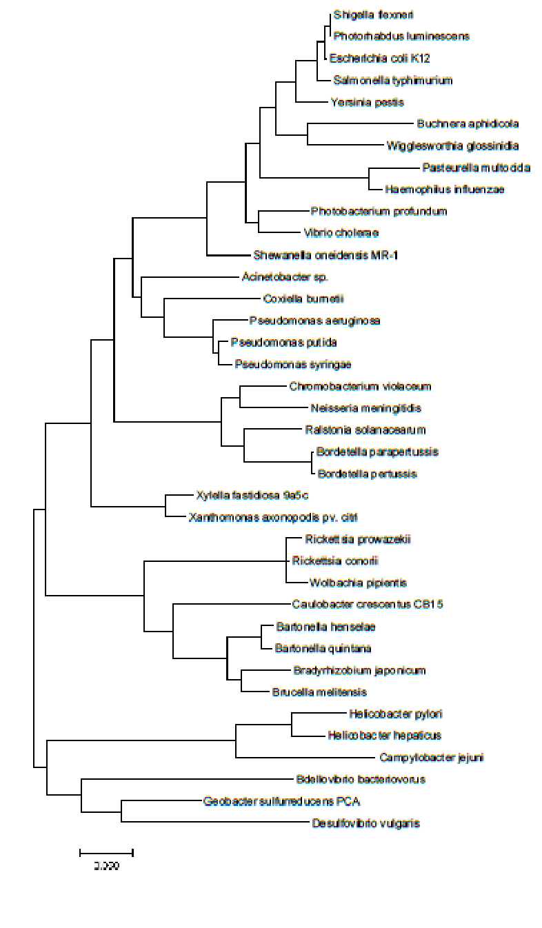
Open the .log file that is included in your .zip bundle from IQ-TREE and find the ‘Best score found’ after finilazing tree search. How does it compare with the model testing best Ln score? Can you explain the difference?
Best-fitting model LogL = -19303.1910
BEST SCORE FOUND LogL = -19284.082
This is still quite a bit better than the best fitting LnL score, probably because during the finalizing tree search a really thorough exploration of tree space has been conducted by IQ TREE, yielding a tree that better fits the data and hence, with higher LnL (the MLE!)
Now compare the best LogL score of your IQ-TREE analysis with the best log likelihood value that you found in MEGA 11 in before. Are they the same?
Using the GTR + Gamma model the LnL value is 11894.34; however using the winning model from the IQ TREE analysis (TN + I + Gamma) this value is 11905.25, which is slightly worse. When repeating these analyses, this time with pairwise deletion the LnL’s become 13869.69 and 13882.63 respectively. In any case, these values are still much higher than those found in the IQ TREE search. The reason for that is probably that both analyses have been based on different number of positions from the same alignment (check in IQ TREE iq.tre files and in the MEGA Captions).
Model |
MEGA |
MEGA |
MEGA |
IQ-TREE |
|---|---|---|---|---|
Pairwise deletion |
Complete deletion |
Use all sites |
||
TN+I+G |
-13858.85 |
-11895.49 |
-19347.05 |
-19303.1910 |
GTR+G |
-13847.07 |
-13858.85 |
-19330.23 |
-19300.0064 |
Once again this shows that LnL values should not be compared between datasets, but between models (or trees) on one and the same dataset!
Why are the LnL values so different among character sets (deletion treatments) but not among models? Using differing number of sites apparently has a large effect on LnL calculation; as indicated above, likelihood values should only be compared from the same dataset. Comparing models has a much smaller effect as only one or two
Why don’t we just go straight to the most complex model, surely that one would fit any data set best? Tempting as it may be, the most complex model will contain the largest amount of parameters, for each of which a value needs to be estimated from the ‘signal’ in the data. There may not be enough signal however to feed all parameters, potentially resulting in imprecise likelihood calculations.
Compare this to the figure in assignment II, above, and discuss any differences, both topological and in terms of nodal support, that you may see. Make sure your rooting is correct, try to find clades in common between your ML tree and the trees in the figure in assignment II; ideally the coloured labels will help you ‘find’ the clades or establish groups are paraphyletic (or even polyphyletic). Also check the bootstrap support for nodes and explore whether they correlate with the length of their branches.
Assignment VI - Optional: Trees are as good as the MSA they’re based on: phylogeny estimation of TDP DNA sequences (60 minutes)
The objective of this assignment is to learn how to use the software package Mesquite for the handling and manipulation of DNA sequence alignments prior to phylogenetic analysis. Mesquite does not (really) build trees, but enables you to optimise alignments, edit character matrices, trace characters over phylogenetic trees, and, quite useful, convert from and to an impressive list of file formats. Mesquite is freeware and can be obtained, along with useful descriptions of tools, here.
TDP-dependent enzyme superfamily
Building a gene tree for a family of enzymes can help to identify how enzymatic functions evolved. The idea is to generate a gene tree including functionally and structurally related sequences from a wide range of taxa, and then I) try to predict function in gene family members that have not been characterised experimentally, and II) infer the evolution of enzyme function itself across the superfamily, including reconstructing ancestral states. Obviously, these questions can only be addressed using a phylogenetic perspective.
The sequence alignment that we used today to illustrate this approach includes 38 γ-Proteobacterial sequences (from [Zvelebil and Baum, 2007]) from well-known enterobacteria such as E. coli, Salmonella and related species. The sequences represent a range of enzymatic functions that are described in Fig. 7.22, below.
The main question now is how to obtain an accurate multiple sequence alignment and this is indeed what this practical will focus on. Although it is not explicitly stated, the alignment given by Zv&B was probably constructed using CLUSTAL, a guide tree-based progressive alignment approach. Whereas this approach is fast and powerful, there are known problems in case of varying levels of sequence conservation along a region to be aligned.
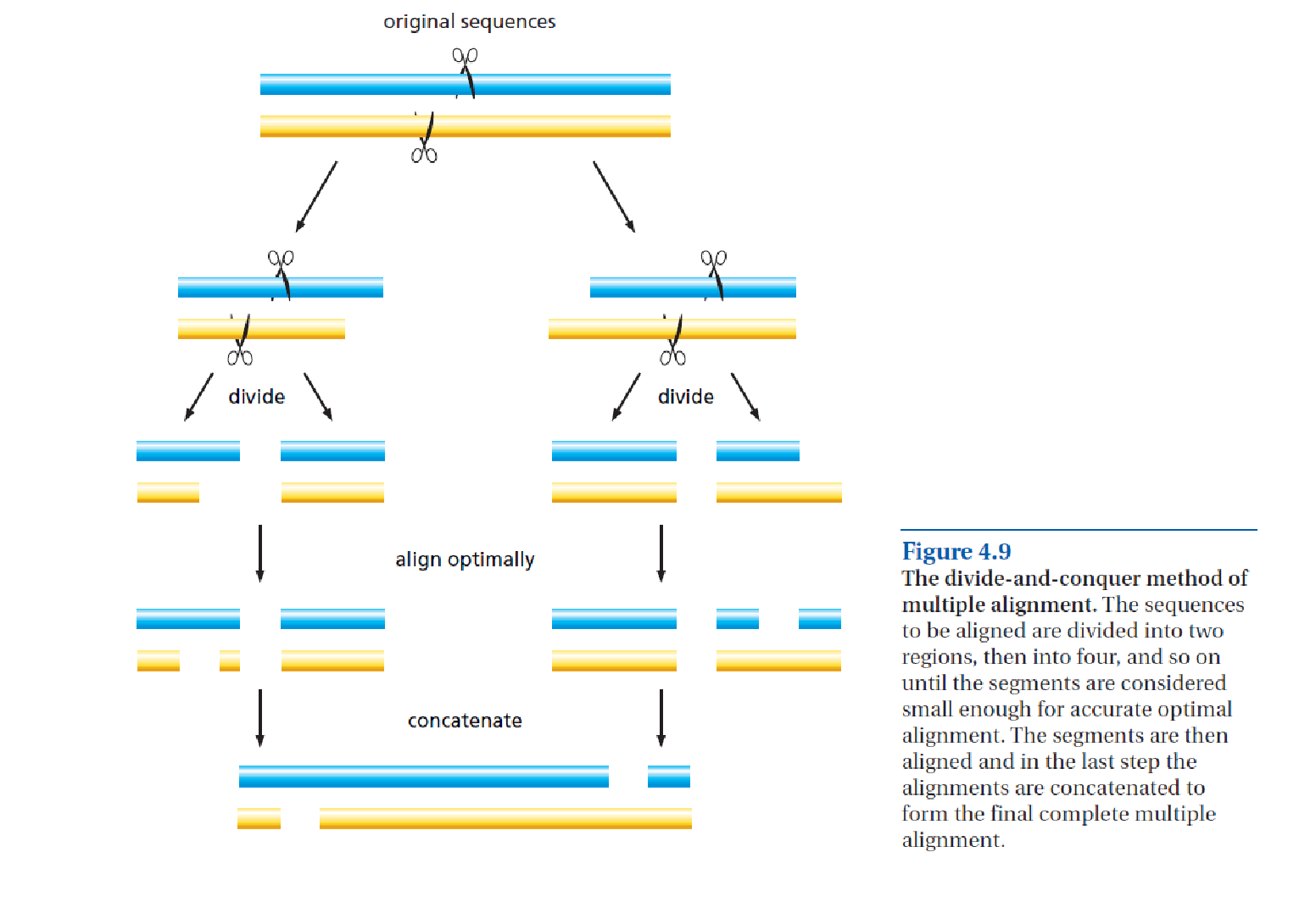
Therefore, in this assignment you will, apart from re-creating the patterns as depicted in Zv&B Figs. 7.22A and B, re-align the sequence matrix using MAFFT, with subsequent phylogenetic analysis and interpretation. MAFFT has a k-mer based approach, allowing ‘breaking-up’ of the sequence into highly-conserved and variable parts prior to alignment, followed by ‘sticking aligned parts together’ afterwards, the divide-and-conquer approach (see Zv&B Fig. 4.9).
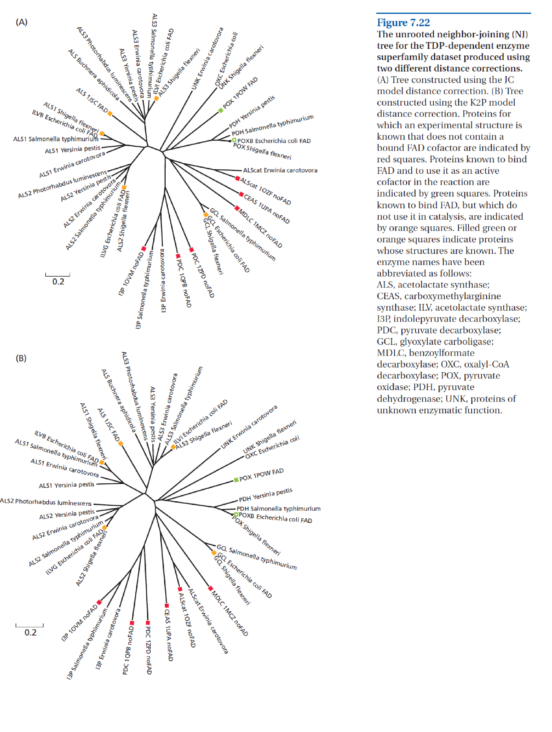
Tasks: Alignment & MAFFT re-alignment
Analyze the TDP-dependent enzyme superfamily sequence matrix (named ‘
TDP_dependent_enzyme_DNA.fas’ which is available from Brightspace, in a similar way to how you analysed the Proteobacterial 16S rRNA sequence alignment in the previous practical. Basically, perform a parsimony analysis and generate a Maximum Likelihood tree using IQ-TREE, withTDP_dependent_enzyme_DNA.fas.For producing an alternative version of the TDP sequence matrix go to MAFFT and upload your TDP .fas file there.
Take a look at all options available but use defaults as set, i.e., do not change any of the settings. Click
Submitand wait, probably a minute or so.You will see some analysis progress information as well as dotplots indicating co-linearity of all sequences. Depending on the load on the server, clicking the
Check nowlink will return your re-aligned sequence alignment.Click
Reformatand select PAUP|NEXUS as Output sequence format, andDownload to fileand clickSubmit.Now start Mesquite which you just installed on your laptop. Once it is ready, open the file you just downloaded from the MAFFT server. Click
Display > Widths > Thin Rowsand selectDisplay > Bird’s Eye Viewin order to get a better view on the alignment.You now want to infer a reading-frame in these sequences, i.e., what are the 1st, 2nd and 3rd codon positions. We do that as follows:
Click
Characters > List of characters.type Ctrl-A in order to select all sites.
Select the column header
Codon positionand thenSet codon position > Minimise stop codons.Return to the Matrix tab.
The sequence alignment is now structured according to codons; in order to visualise this more clearly select
Display > Color Matrix Cells > Color nucleotide by amino acid.Click
Display > Show Color Legendin order to interpret the amino acid-level patterns. Ideally, no or only a few stop codons (black) should show.Save this file under a logical name and give it the
.nexextension (for nexus file format). Also selectFile > Save Matrix as PDFand save to your own space.Select
File > Export > Simplified NEXUSso that this MAFFT-aligned matrix can be imported in IQ-TREE.
Tasks: Comparing original vs. MAFFT IQ-TREES and clade support
Now that you have two versions of the TDP sequence matrix you can start comparing the tree-topological results. Therefore, perform the parsimony analysis and IQ-TREE ML analysis as described above for the Proteobacterial practical now for the MAFFT re-aligned matrix, in the Simplified NEXUS format.
Compare the actual MSAs by performing Task 6-9 (previous page) again, with the original TDP sequence matrix. Save a .pdf of the matrix as you did for the MAFFT re-aligned matrix. Compare the two .pdfs, by ‘visual inspection’ and discuss which one you would consider a ‘better alignment’.
Make sure to compare an IQ-TREE from the original with an IQ-TREE from the MAFFT re-aligned analysis and discuss the differences.
You will have noticed that in Zv&B Figs. 7.22A and B no bootstrap support values are given, but you will have these now in your IQ-TREEs. Interpret bootstrap clade support in your IQ-TREES and discuss whether the claims by Zvelebil & Baum with regards functional evolution are supported, or to what extent we can be confident about them.
Original:
MAFFT:

Original, IQ-TREE:
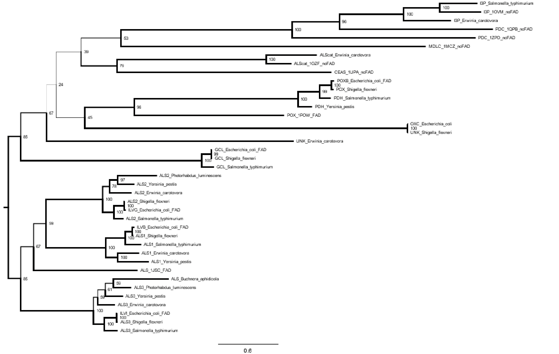
MAFFT alignment, IQ-TREE:

Assignment VI answers
Compare the two .pdfs, by ‘visual inspection’ (this may cause your PC to slow down for a minute, have patience…) and discuss which one you would consider a ‘better alignment’. One could argue that the MAFFT alignment is better, because of the divide-and-conquer approach: first align conserved ‘anchors’ across all terminals, then do the bits in between. Visual inspection of the two alignment versions seems to suggest the MAFFT-alignment looks more ‘quiet’ which would be consistent with fewer substitutions -because better alignment.
You will have noticed that in Zv&B Figs. 7.22A and B no bootstrap support values are given, but you will have these now in your IQ-TREEs. Interpret bootstrap clade support in your IQ-TREES and discusswhether the claims by Zvelebil & Baum with regards functional evolution are supported, or to what extent we can be confident about them.
One could argue that the deeper nodes in our IQ-TREE analysis appear to be poorly supported, with bootstrap values < 80% in several cases. Interpretation by Zv&B with regards duplication events in the ALS genes are more or less supported by the bootstraps; the topology in the rest of the tree is fairly poor and should probably better be represented by a polytomy.
This means that the position of Erwinia carotovora, for which Zv&B state: “From its position, it will probably function in a similar way to either OXC or pyruvate oxi dase (POX), although it is also not far from the glyoxylate carboligase (GCL) cluster.” But this is hard to support given the poor nodal support in this part of the tree, meaning its position is unsecure and could actually go in various places on this part of the tree.
Project Preparation Exercise
Using last chapter’s ARF multiple sequence alignment (amino acid sequence), aligned in MAFFT, now use MEGA 11 in order to make a NJ tree, using the Poisson and then the Dayhoff model of amino acid substitutions.
Use FigTree to make a proper tree picture; then generate a Maximum likelihood tree (with bootstraps) in IQ-TREE, and produce its pretty picture in FigTree.
Is the tree properly rooted? What outgroup could be added in case it is not present yet?
Describe the following items in a few bullet points each. You may include up to two figures or tables.
Materials & Methods What did you do? Which data, databases and tools did you use, and why did you choose them? What important settings did you select?
Results What did you find, what are the main results? Report the relevant data, numbers, tables/figures, and clearly describe your observations.
Discussion & Conclusion Do the results make sense? Are they according to your expectation or do you see something surprising? What do the results mean, how can you interpret them? Do different tools agree or not? What can you conclude? Make sure to describe the expectations and assumptions underlying your interpretation.
References#
- 3W1
J. Huerta-Cepas, M. Marcet-Houben, and T. Gabaldón. A nested phylogenetic reconstruction approach provides scalable resolution in the eukaryotic tree of life. PeerJ PrePrints, 2014. URL: https://peerj.com/preprints/223/, doi:10.7287/peerj.preprints.223v1.
- 3W2
J. Hadfield, C. Megill, S.M. Bell, J. Huddleston, B. Potter, C. Callender, P. Sagulenko, T. Bedford, and R.A. Neher. Nextstrain: real-time tracking of pathogen evolution. Bioinformatics, 34(23):4121–4123, 05 2018. doi:10.1093/bioinformatics/bty407.
- 3W3(1,2,3,4,5,6,7,8,9,10,11,12,13,14,15,16,17,18,19,20,21,22,23,24,25,26)
Dick de Ridder, Anne Kupczok, Rens Holmer, Freek Bakker, Justin van der Hooft, Judith Risse, Jorge Navarro, and Tomer Sardjoe. Self-created figure. 2024.
- 3W4
DataBase Center for Life Science (DBCLS). Animal illustrations. 2023. URL: https://togotv.dbcls.jp/pics.html.
- 3W5
DataBase Center for Life Science (DBCLS). Animal illustrations. 2021. URL: https://togotv.dbcls.jp/pics.html.
- 3W6
J. Heled and A.J. Drummond. Bayesian inference of species trees from multilocus data. Molecular Biology and Evolution, 27(3):570–580, 11 2009. doi:10.1093/molbev/msp274.
- 3W7(1,2,3,4)
K. Tamura, G. Stecher, and S. Kumar. Mega11: molecular evolutionary genetics analysis version 11. Molecular Biology and Evolution, 38(7):3022–3027, 04 2021. doi:10.1093/molbev/msab120.
- 3W8
A1. Collapsedtreelabels-simplified. 2009. URL: https://commons.wikimedia.org/wiki/File:CollapsedtreeLabels-simplified.svg.
- 3W9
A. Mimi. William of ockham (1285 - 1347). english philosopher, also known as the "invincible doctor" (doctor invincibilis) and the "venerable initiator" (venerabilis inceptor). 2022. URL: https://commons.wikimedia.org/wiki/File:GUILHERME_DE_OCCAM_(1285_-_1347)._Fil%C3%B3sofo_ingl%C3%AAs,_tamb%C3%A9m_conhecido_como_o_%22doutor_invenc%C3%ADvel%22_(Doctor_Invincibilis)_e_o_%22iniciador_vener%C3%A1vel%22_(Venerabilis_Inceptor),.jpg.
- 3W10
Tony Hodge and M. Jamie T. V. Cope. A myosin family tree. Journal of Cell Science, 113(19):3353–3354, 10 2000. doi:10.1242/jcs.113.19.3353.
- 3W11
Bui Quang Minh, Heiko A Schmidt, Olga Chernomor, Dominik Schrempf, Michael D Woodhams, Arndt von Haeseler, and Robert Lanfear. Iq-tree 2: new models and efficient methods for phylogenetic inference in the genomic era. Molecular Biology and Evolution, 37(5):1530–1534, 02 2020. doi:10.1093/molbev/msaa015.
- 3W12(1,2)
M. Zvelebil and J.O. Baum. Understanding Bioinformatics. Garland Science, London, United Kingdom, 2007. ISBN 9780203852507. doi:10.1201/9780203852507.
._Fil%C3%B3sofo_ingl%C3%AAs,_tamb%C3%A9m_conhecido_como_o_%22doutor_invenc%C3%ADvel%22_(Doctor_Invincibilis)_e_o_%22iniciador_vener%C3%A1vel%22_(Venerabilis_Inceptor),.jpg)