Protein structure prediction

4. Protein structure prediction#

– Justin van der Hooft

Predicting protein structures: the sequence-structure-function paradigm#

A lot of sequences have become available. However, for most, we do not yet know what type of proteins they represent, and what functionality they have.

Proteins are essential for life on earth. They have many kinds of functions in organisms such as supporting its structure (e.g., keratin in our skin), performing enzymatic reactions (e.g., Ribulose-1,5-bisphosphate carboxylase-oxygenase, a.k.a. Rubisco, in plants), or receptors for transduction of signals that mediate cell-to-cell communication. As discussed in chapter 1, only a relatively small amount of amino acid building blocks forms the basis of a structurally very diverse protein repertoire. Hence, to understand the function of proteins, knowing their structures is key. In chapter 1 you have also learned that proteins are created as a long chain of amino acids held together by peptide bonds, i.e., a polypeptide chain (the primary structure), that folds into a three-dimensional (tertiary) structure, based on various types of interactions between amino acid side groups. Usually, during this folding process, shorter stretches of local 2D (secondary) structures form first, held together by hydrogen bonds. Interestingly, whereas the amino acid sequence of proteins may differ, their folding may still result in comparable 3D structures of the polypeptide chain – with comparable or even similar functionality (see Fig. 4.1). Several folded polypeptide chains can form the final quaternary complex that is functional within the cell. Thus, the protein folding process is important, as it determines the 3D structure of polypeptide chains, and misfolding can lead to misfunctioning of the protein, for example by non-specific binding to other proteins, causing a disease in humans, or a less-performing mutant in plants.

Fig. 4.1 Protein structures of human myoglobin (top left), African elephant myoglobin (top right, 80% sequence identity to human structure analogue), blackfin tuna myoglobin (bottom right, 45% sequence identity to human analogue), and pigeon myoglobin (bottom left, 25% sequence identity to human analogue). Myoglobin can be found in muscles and its main function is to supply oxygen to muscle cells. The protein structures in this figure illustrate how structure can be largely the same even for sequences that are quite different. Credits: [Rubiera, 2021].#

While current experimental methods can generate many sequences of hypothetical proteins present in organisms, it is still hard and expensive to determine the corresponding 3D protein structures experimentally. The main traditional experimental analytical techniques used are nuclear magnetic resonance (NMR) spectroscopy and X-ray crystallography. The former yields useful but often noisy measurements with usually multiple structural conformations; whereas the latter is more accurate, but easily costs 120,000 euros. Furthermore, it can take a year or even longer to fully elucidate the protein 3D structure from the data, and some structures cannot be measured at all, for example due to crystallization problems. Fortunately, fueled by recent technical advances, biological sequence data has become widely available, mostly in the form of genomic sequences. By translating these DNA sequences into possible amino acid sequences using the codon language you have learned about in chapter 1, amino acid sequences can be inferred in which theoretical proteins can be predicted. However, the sheer number of biological sequences make manual analysis of such predicted protein sequences too daunting. Thus, alternative methods to derive 3D protein structures are needed to interpret the large amount of biological sequence data that has become available in the recent decades. Consequently, predicting protein structures based on protein sequence information has been a topic of high interest and relevance to biochemists and scientists in general for many decades.

The sequence-structure-function paradigm states that, in principle, all information to predict the folding of a protein, and thus its 3D structure and ultimately its function, is stored in its primary sequence. In practice, however, predicting structure from its sequence turned out to be a very complex and challenging task. One of the reasons for this complexity is due to the both short- and long-range interactions between protein local structure elements, i.e., interactions between secondary structure (2D) elements such as sheets and helices typically form anchor points upon which the tertiary (3D) structure is based. This chapter first describes 2D structure assignment and prediction, after which foundational 3D structure prediction approaches are discussed, including the main challenges and the three zones of tertiary structure prediction. It ends with the most recent approaches to predict and compare tertiary structures: AlphaFold and Foldseek.

Secondary protein structure prediction#

Proteins consist of several locally defined secondary structure elements of which alpha helices (α-helices) and beta strands/sheets (β-strands/sheets) are the most commonly occurring ones. Please note here that a β-strand refers to one side of the β-sheet, where two strands come together to form the sheet structure. In this section, we will cover how to assign these two secondary structure elements using 3D protein structures, and how to predict these secondary structure elements based on sequence data. Furthermore, we will cover the prediction of two biologically relevant “special cases” of secondary structure elements: transmembrane sections and signaling peptides.

Secondary structure assignment#

If we consider the 3D structure of folded protein chains, we typically observe that the more ordered parts of their structures usually contain more α-helices and β-strand stretches than the more randomly organized parts. As these elements fold locally, they can initiate folding of more complex tertiary folding patterns. Indeed, the presence/absence of α-helices and β-sheets and their specific conformation helps to categorize proteins. As a result, databases exist that categorize proteins according to specific fold types, in a structured, hierarchical way. Therefore, the assignment of amino acid residues to either α-helix, β-strand, or “random coil” (i.e., “other”), based on the 3D structure of a protein chain, can be seen as a first step to understand the protein structural configuration. Also, when we need training data to predict secondary structure elements based on the primary (1D) sequence, we would need sufficient labeled training data based on actual assignments. Hence, several assignment tools were developed to replace the previously discussed daunting task of manual assignment of secondary structure elements based on known 3D information.

The three options for an amino acid residue as mentioned above would translate into a so-called “three-state model”, (α-helix, β-strand, or other) used by secondary structure assignment tools such as DSSP, PALSSE, and Stride, that use 3D structures as an input to assign three secondary structure labels. You will get hands-on experience with the interpretation of the outcome of these tools during the practical assignments. Please note that there are additional – less occurring – secondary structure elements that could be recognized, such as the β-turn, a sharp bend in the protein chain, and several special helices. As a result, some tools will return eight states or even more. However, these can also be grouped in the three original states listed above.

Assigning or predicting the secondary structure of a protein is only useful if you have an idea of the accuracy of the assignments/predictions from a given program. The measured accuracy is used to help estimate its likely performance when presented with a sequence of an unknown structure. Accuracy can be measured either in respect of individual residue predictions or in relation to the numbers of correctly predicted helices and strands. One commonly used and relatively straightforward method to assign accuracy to individual residues is the Q₃ measure. The values of Q₃ can range between 0 and 100%, with 100% equalling a perfect prediction. The value for a completely at random prediction depend on the number of different labels or “states” we predict: if we predict in the “three-state model”, a random prediction would return 33% for Q₃. Please note that the same value can mean completely different things (Fig. 4.2); hence, the values need to be considered together with the actual sequence aligments. Whilst it may seem natural to strive for a perfect prediction, the maximum Q₃ that is generally achievable is ~80%. This is mainly caused by difficulties in defining the start and end of secondary structure elements: the different tools that assign or predict secondary structure may well deviate at the borders of the predicted elements. Even as a human, manual annotation of secondary structure elements may pose challenges on which residues are inside or outside secondary structure elements. During the practical assignments, you will explore this phenonemon more.

Fig. 4.2 The Q₃ measure produces useful accuracy predictions when the resulting secondary structure prediction contains a slight shift compared to the actual structure (prediction 1). It is however not useful when the secondary structure elements have been interpreted incorrectly (E -> H in prediction 2). Credits: CC BY-NC 4.0 [de Ridder et al., 2024].#

Secondary structure prediction#

Here, we will describe approaches to predict secondary structure elements on the basis of sequence data alone. As these approaches form the foundation for tertiary structure prediction tools, it makes sense to study them first.

One of the first methods to predict secondary structures used statistics to infer a residue’s secondary structure and was the so-called Chou-Fasman approach that, starting in the 1970s, used an increasing set of reference protein 3D structures and 2D structure assignments to determine the natural tendency (propensity) for each amino acid type to either form, break, or be indifferent to form or break an α-helix or β-strand (see Fig. 4.3). If we consider a stretch of amino acids, these propensities help to determine if and where an α-helix or β-strand starts or stops. For example, some amino acids have a strong tendency to form α-helices (e.g., Alanine) or β-strands (e.g., Isoleucine), whereas others tend to break these local structures. In particular, we can observe that Proline is a strong breaker of both structure elements. This can be explained by the special side group arrangement of Proline: this is fused twice to the backbone of the protein, rendering the amino acid very inflexible when it comes to the phi (φ) and ψ (psi) angles it can render (see chapter 1 for more information on phi and psi angles). Another amino acid that that tends to break alpha helices and beta strands is Glycine. Whilst now superseded, first by more accurate statistical methods and more recently by machine learning-based methods, the Chou-Fasman approach very elegantly demonstrates how the side groups of amino acids impact their tendency to form specific structures.

Fig. 4.3 Chou and Fasman Propensities §. F stands for strong former, f weak former, while B and b stand for strong and weak breaker, respectively. I (indifferent) indicates residues that are neither forming nor breaking helices or strands. We can see that Pro has the lowest propensity for forming a helix and a low one for strands as well. However, many other residues that are either weak or indifferent have been reclassified since the propensities shown here have been reparameterized as more data have become available. Credits: CC BY-NC 4.0 [de Ridder et al., 2024].#

In subsequent decades, several statistical-based methods were developed that improved sequence-based predictions of secondary structure elements. They, for example, started to include information of multiple sequence alignments including residue conservation: such approaches first matched the query sequence to database sequences with known 3D structures and assigned secondary structure elements. Then, using the best matching sequences, the secondary structure state of amino acid residues of the query sequence stretch are inferred by averaging the states from the homologous sequences found, further adapted using additional information such as the conservedness of the residue. An example of such an approach is Zpred. In general, the use of multiple sequences and additional information about the amino acid residue’s physicochemical properties and conservedness greatly enhanced the prediction performance. Next, machine learning took over in the form of neural networks. Such approaches use a so-called sliding window that encompass multiple amino acid residues of which the central one’s state is predicted using a model. They typically result in probabilities for each state that can be used to assign the most likely state, i.e., alpha-helical, beta-strand, or random coil (in a three-state model). Examples of such approaches are Jnet and RaptorX.

Most recently, deep learning approaches have been introduced to predict secondary structure elements based on sequence information. The state-of-the-art approach is NetSurfP, of which version 3 is currently running. You will gain hands-on experience with NetSurfP 3.0 during the practical assignments. Here, we will briefly explain how it works and how to assess its results. The prediction tool uses a deep neural network approach to accurately predict solvent accessibility and secondary structure using both three- and eight-state definitions, amongst other properties. To make this approach work, sufficient training data is needed of protein chains with known PDB 3D structures. To avoid over-fitting the model on predominant sequence stretches, each protein sequence that had more than 25% sequence identity to any other protein sequence already in the test set was removed. To ensure good quality data, a resolution of 2.5 Angstrom or better was selected for. This resulted in ~10,000 protein sequences used for training. To obtain “ground truth”, DSSP was used (see Secondary structure assignment) to calculate properties such as solvent accessibility and secondary structure states, resulting in a labeled data set for training. The parameters of the neural network were trained using small batches of protein sequences and their “ground truth” to result in a final model.

Fig. 4.4 NetSurfP 3.0 output for a yeast protein that contains both α-helical as well as β-strand sections. Credits: [Høie et al., 2022]. The 3D structure of this protein was obtained from: [Eswaramoorthy et al., 1999].#

As we have seen in chapter 1, there are key similarities and differences between α-helices and β-sheets. Both secondary structure elements rely on hydrogen bonds between backbone atoms in the polypeptide chain. However, where residues involved in α-helices only have local interactions in the chain, β-sheet residues can have long-range interactions. Consequently, β-sheets are more difficult to predict for sequence-based prediction tools. The availability of sufficient homologous proteins can alleviate this bottleneck and provide reliable predictions of β-sheets as well. Also, the development of 3D structure prediction tools (see Tertiary protein structure prediction) is expected to lead to further improvements in predicting secondary structure elements and other per-residue properties like surface exposure/solvent accessibility based on sequence information alone.

Transmembrane protein sections#

Cells are surrounded by a membrane that consists of a lipid bilayer. The membrane is literally what separates the inside of the cell with the outside world. Hence, if messages need to be passed on from outside to inside the cell, or vice versa, these messages will need to pass the apolar environment of the membrane. To do so, the cellular machinery is using proteins to assist in signal transduction across the membrane. Where globular proteins are present within the cell, so-called transmembrane proteins span the membrane at least once. It is estimated that ~30% of the proteins are transmembrane, indicating their functional importance. Due to restrictions of the protein exterior put on by the specific environment of the membrane in terms of size and polarity, only some local structural configurations are typically found to span the membrane. These configurations are typically linked to the protein’s function: be it a receptor for signal transduction or a transporter of specific substances across the membrane.

Let us consider size first: the average thickness of a membrane is ~30 angstrom (Å), which corresponds to an α-helix of between 15 and 30 residues to make it fit within the membrane layer.

Three different types of transmembrane proteins

Fig. 4.5 Schematic representation of proteins with transmembrane sections, also called transmembrane proteins, with the membrane represented in light yellow: 1) an alpha-helix containing protein spanning the membrane once (single-pass) 2) an alpha-helix containing protein spanning the membrane several times (multi-pass) 3) a multi-pass membrane protein containing β-sheets. Credits: CC BY 2.5 [Foobar, 2006].#

The simplest local transmembrane element is an alpha-helix of ~ 15-30 amino acid residues with mainly apolar side groups (Fig. 4.5, 1). The length is restricted by the length of the lipid bilayer, whereas the apolar side groups will have favorable interactions with the acyl chains of the lipids in the membrane. A transmembrane protein can span the membrane one or more times (i.e., Fig. 4.5, 1 & 2), and in some cases a special configuration of the transmembrane proteins creates a “pore”-like structure. Here, some helical residues can be charged as the pore environment is completely shielded from the membrane bilayer. Another commonly used transmembrane configuration is the “beta-barrel”. This element consists of 8 – 22 transmembrane β-strands (although larger ones with even more β-strands may well exist) that together form a “barrel shape” (Fig. 4.5, 3), effectively separating the inside of the barrel from the outside, thereby creating a pore in the membrane. Such pores can be sealed off with a “switch” in the form of a protein stretch that is either in the “open” or “closed” configuration.

Signaling peptides#

The place where proteins are built in the cell is usually not where they act. To exert their function at the right place, proteins need to be transported from where they are folded and formed. The cellular machinery has developed a signaling system that use “peptide tags” to enable effective transport of polypeptide chains to their site of action prior to becoming active. Such “tags” are called signal peptides that are peptide recognition signals for the cellular transporter machinery. Typical sites of actions for which signal peptides exist include the cell membrane and the endoplasmic reticulum. Furthermore, signal peptides can steer proteins to be secreted from or imported into lysosomes. Hence, the presence of such a signal peptide can provide important clues as to what the site of action of a protein may be based on its amino acid sequence.

The signal peptide is an N-terminal leader amino acid sequence that consists of ~ 15-30 residues added to the N-terminus of the mature protein (Fig. 4.6). The actual recognition of signal peptides by the cellular transporter machinery is not based on a conserved amino acid sequence, but it largely depends on the physicochemical properties of the amino acids in the signal peptide. A signal peptide typically consists of three regions: the first region (the n-region) usually contains 1–5 positively charged amino acids, the second region (the h-region) is made up of 5–15 hydrophobic amino acids, and the third region (the c-region) has 3–7 polar but mostly uncharged amino acids.

Signal sequence (signal peptide) with a hydrophobic core-region (h) and hydrophilic N- (n) and C-terminal (c) flanking regions

Fig. 4.6 Schematic representation of a signal peptide and its positively charged N-terminal, hydrophobic core-region (h-region), the polar (mostly) uncharged c-region, and the mature protein (o). Credits: CC BY-SA 3.0 modified from [Yikrazuul, 2010].#

Sequence-based prediction of transmembrane sections and signal peptides#

Given their functional clues, the prediction of transmembrane sections and signal peptides based on amino acid sequence alone is very advantageous when studying the possible functions of unknown proteins. DeepTMHMM is currently the top-performing tool to predict transmembrane sections and signaling peptides in protein sequences. The program predicts several labels for each amino acid in a sequence: signal peptide (S), inside cell/cytosol (I), alpha membrane (M), beta membrane (B), periplasm § and outside cell/lumen of ER/Golgi/lysosomes (O).

Both transmembrane sections and signal peptides are largely defined by the physicochemical properties of the amino acid residues that they constitute, rather than a conserved motif or short sequence of residues. This makes it very hard to recognize these secondary structure elements using classical methods based on alignment. Using machine learning methods, however, the characteristics of a training data set with known sequences can be learned and used for the prediction of unknown data. The trained models can subsequently judge the properties of amino acids in unknown sequences, thereby allowing the recognition of transmembrane sections and signal peptides. Hence, DeepTMHMM uses a deep learning model that takes a protein sequence as input, and then outputs the corresponding per-residue labels. Taken all together and considering their order within the amino acid sequence, the residue labels define the predicted topology of the protein. DeepTMHMM can predict five different topologies, namely alpha helical transmembrane proteins without a signal peptide (alpha TM), alpha helical transmembrane proteins with signal peptide (SP + alpha TM), beta-barrel transmembrane proteins (Beta), globular proteins with signal peptide (SP + Globular) and globular proteins without signal peptide (Globular). Importantly, the two secondary structure elelements predicted here share properties and the deep learning model needed sufficient example data to differentiate transmembrane sections from signal peptides.

In Fig. 4.7 you can observe a typical output of DeepTMHMM - alpha TM for a multi-pass transmembrane protein.

An example output of DeepTMHMM - alpha TM

Fig. 4.7 Left, output of DeepTMHMM - alpha TM prediction on Bovine Adhesion G protein-coupled receptor G7 (ADGRG7, A4IFD4). Right, a gff file of the same protein where the number of transmembrane structures (α-helices), their amino acid positions, and whether the residues are inside or outside the membrane indicated. Credits: [Hallgren et al., 2022].#

Fig. 4.8 shows an example output of DeepTMHMM - beta for a beta-barrel transmembrane protein.

Fig. 4.8 Left, output of DeepTMHMM - beta prediction on the outer membrane protein C (precursor) of Salmonella typhimurium (OMPC-SALTY, P0A263). Right, a gff file of the same protein where the signal peptide position, the number of transmembrane structures (β-sheets), their amino acid positions, and whether the residues are in the periplasm or outside the membrane indicated. Credits: [Hallgren et al., 2022].#

SignalP#

In the previous section it was covered how DeepTMHMM can be used to predict the presence of signal peptides; however, more dedicated tools exist for the discrimination between signal peptides types, such as SignalP 6.0. This tool can predict signal peptides from sequence data for all known types of signal peptides in Archea, Eukaryota, and Bacteria. Additionally, SignalP 6.0 predicts the regions of signal peptides. Depending on the type, the positions of n-, h- and c-regions as well as of other distinctive features are predicted.

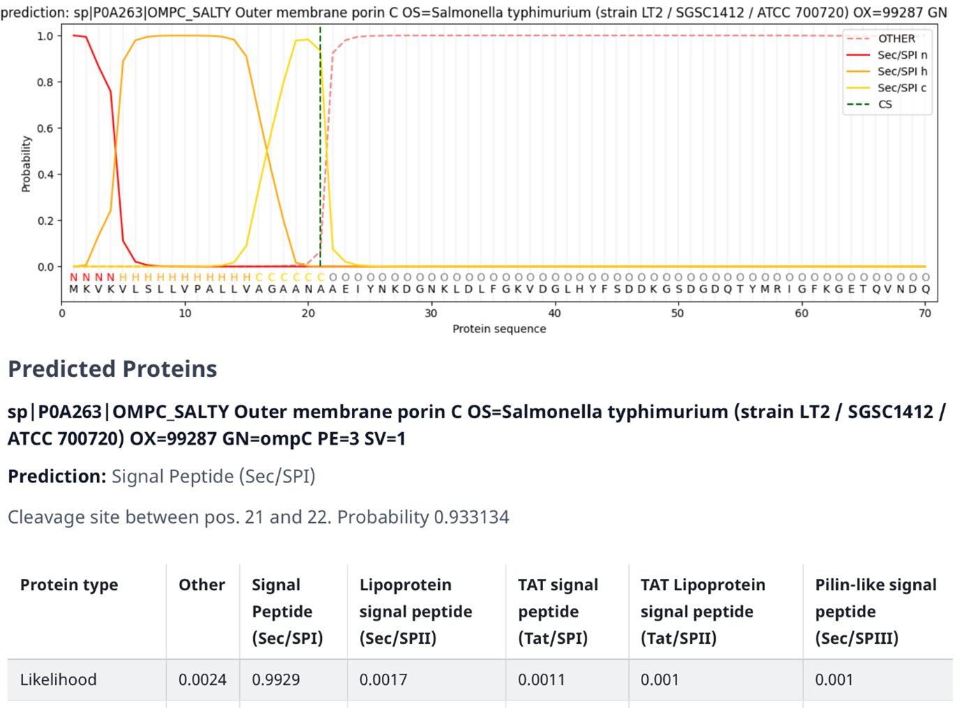
Fig. 4.9 SignalP output on the outer membrane protein C (precursor) of Salmonella typhimurium (OMPC-SALTY, P0A263). Credits: [Teufel et al., 2022].#

In Fig. 4.9 an example output of SignalP 6.0 is shown (note the resemblance of the structure of the signal peptide to Fig. 4.6). The figure contains several elements:

The graph at the top consists of the following elements:

The dark orange line (Sec/SPI n) indicates the probability of a specific region being identified as the N-terminus, which is also displayed as the letter “N” underneath the line.
The light orange line (Sec/SPI h) indicates the probability of a specific region being identified as the h-region, which is also displayed as the letter “H” underneath the line.
The yellow line (Sec/SPI c) indicates the probability of a specific region being identified as the c-region, which is also displayed as the letter “C” underneath the line.
The dashed orange line (OTHER) indicates the probability of a specific region being identified as something other than the signal peptides subsections, such as the mature protein itself. This is also displayed as the letter “O” underneath the line.
The dashed green line (CS) indicates the probability of a specific region being identified as the cleavage site.
The protein sequence underneath the letters that indicate which section a region belongs to.

The signal peptide score (the orange lines) is trained on the differentiation of signal peptides and other sequences and has a high value if the corresponding amino acid is part of the signal peptide. Therefore, amino acids of the mature protein have a low signal peptide score. The maximum cleavage score (the dashed geen line) occurs at the position of the first amino acid of the mature protein, so one position behind the cleavage site. The cleavage score analysis was trained on the recognition of the cleavage site between signal peptide and the protein sequence.

The standard secretory signal peptide is called Sec/SPI and it is transported by the Sec translocon and cleaved by Signal Peptidase I (Lep). There are four other signal peptide types (see, see also box below) but they are beyond the scope of this course. However, it is important to know that tools like signalP are able to distinguish between the different signal peptide types and make accurate predictions about their probabilities.

The information below the graph consists of the following elements:

The prediction indicates the most probable type of signal peptide for the given sequence.
The cleavage site shows the amino acid location in the protein sequence where the cleavage site is located, as well as its probability.

The table at the bottom of the page consists of the following elements:

Likelihood/probability scores for the different types of signal peptides and the chance of it not being a signal peptide at all (Other).

Tertiary protein structure prediction#

First, it is good to realize that the prediction of secondary structure elements has formed the foundation of tools that predict 3D structures of proteins. We will first explore the three traditional structure prediction approaches, which will be followed up by the most prominent new approach in structure prediction (AlphaFold) that relies on several concepts of the traditional approaches.

Fig. 4.10 The three zones of tertiary structure prediction approaches. Credits: [CC BY-NC 4.0] [de Ridder et al., 2024].#

Various approaches including ab initio, threading (also called fragment-based modelling), and homology modelling have been proposed and used to go from sequence to structure, with both sequence identity and alignment length as the most important factors to decide which approach to choose. To make an effective choice between these three traditional structure prediction approaches, the so-called three zones were introduced (Fig. 4.10). According to the figure, as we can observe, below 20% sequence identity between the query protein sequence and sequences with experimentally derived structures, one needs to refer to ab initio approaches, literally translating as: from the start. As such approaches are computationally heavy and as they also require a lot of expert knowledge, they are not widely used. In essence, such approaches aim to model the protein sequence folding process using physicochemical properties of the amino acid residues and their surroundings. As the sequence length increases, ever-increasing possible folds occur for the entire 3D structure, making it a computationally intensive task. For example, consider 100 amino acid residues that each have their psi, phi, and omega angles. If they would (only) have have 3 possibilies per angle, this would lead to 3^300 (= 10^143) possible folds for the sequence. If each fold would take just 1 second to assess its likelihood to be realistic and energy-favorable, it would take us 10^126 years to analyze and come up with a suggested 3D structure, and that is just 100 amino acids under severe contraints.

Fortunately, the database of experimentally derived protein 3D structures is constantly growing. Therefore, there is a good chance of having >20% sequence identity of your query sequence. As we can see in Fig. 4.10, the length of the sequence alignment is another crucial factor: if a shorter stretch is matching, the threading (or fragment-based) approach can be used. This approach focuses on matching these stretches to known folds, i.e., local structure often consisting of secondary structure elements. This can already help to hypothesize on the protein’s function, if a functional domain is matched to the query sequence. As this approach is also relatively computationally demanding, and newer approaches as discussed below (i.e., AlphaFold) excel in recognizing such folds, we will not gain practical experience with the approach during this course.

If both the query sequence identity and length of the alignment are large enough, homology modelling can be attempted to create a structure model. So-called “template sequences” have to be found in the protein structure database that are “similar enough” to serve as a structural blueprint for the 3D prediction.

Nowadays, SWISS-MODEL provides precalculated 3D homology models. It is important to note that SWISS-MODEL now also contains the AlphaFold deep learning-based models (see AlphaFold section). Hence, it is important to notice the origin of the 3D structure models, and all will need to be evaluated on their reliability. You will learn how to do that for homology modelling during the practical assignments.

Still, new protein sequences that bear almost no resemblance to existing ones are discovered almost every day. Hence, the scientific community has been adopting various artificial intelligence-based approaches of which AlphaFold is the most prominent one to date.

AlphaFold#

Protein structures in the Protein Data Bank

Fig. 4.11 Top: Number of unique 3D protein structures (based on their sequence) at 95% sequence identity that have been added annually to the Protein Data Bank from 1976 – present time. Bottom: Number of 3D protein structures that have been added to the Protein Data Bank from 1976 – present time. Note: the low number of structures in 2024 is caused by these statistics being taken from PDB early in the year, meaning many more structures are likely to be generated over the rest of 2024. Credits: CC BY 4.0 [Berman et al., 2024].#

Recently, the DeepMind team of Google introduced a machine learning-based approach called AlphaFold. This reader describes how AlphaFold builds on previous approaches and has already had substantial impact in biochemistry and bioinformatics. An analogy could be made to the introduction of the smartphone: whereas previously, one needed to go to the library to find a computer and connect to the internet to get to a weather forecast, one now simply takes the phone and looks up the weather. The reader explains why AlphaFold could be developed and work only now, how it was compared to other approaches in a fair manner, how it relies on database search and multiple sequence alignment, and what the introduction of the AlphaFold Protein Structure Database (AlphaFold DB), that contains AlphaFold-predicted structure models, means for discovery pipelines.

It is good to realize why AlphaFold could work in the first place. The AlphaFold approach is based on machine learning, i.e., computer algorithms that fit a predictive model based on training data. Such a model can then predict the structure, when given a sequence that it has not seen before. DeepMind made use of very large neural network models, so-called deep learning. The training data for such models ideally consists of many known examples for very complex problems such as protein structure prediction. The Protein Data Bank (PDB) collects such experimental training data, i.e., measured protein 3D structures. By now, ~218,000 PDB entries are available of ~150,000 unique protein sequences at 95% sequence similarity (Fig. 4.11, top). The latter number is important, as a sufficiently diverse set of examples will ensure that there are enough examples in the training data to recognize relevant patterns of various protein folds and other structural features.

As input for their most recent machine learning model, the DeepMind team predicted the structure of 100,000 protein sequences and added those to the training data, a technique called data augmentation. Thus, at the time of model training, the team could use around 300,000 protein sequences - 3D structure combinations to train their AlphaFold model that uses a FASTA file as input and outputs a 3D structure model that is described in the Assessing a protein structure model quality section.

The impact of AlphaFold on biochemistry#

The true impact of AlphaFold would be difficult to assess without an independent test. Since protein folding and 3D structure prediction is one of the grand challenges of biochemistry, the Critical Assessment of protein Structure Prediction (CASP) competition was founded in 1994. CASP is a community-wide competition where research groups are required to predict 3D structures from protein sequences that do not have any public 3D structure available. More than 100 research groups worldwide join the CASP competition every two years. Using all sequence and structure data available at the present time, they predict structures for protein sequences with newly derived (yet unreleased) structures, specifically withheld from the public for the purpose of this competition.

AlphaFold progress; Amino acid residue in protein backbone

Fig. 4.12 Left: Average GDT tests of the contest winners. Right: Schematic view of amino acid residue in protein backbone with key atoms labelled, including the alpha carbon used for GDT-TS. Credits: Left: [Callaway, 2020] and right: CC BY-SA 3.0 [LociOiling, 2018].#

The left side of Fig. 4.12 shows both the progress the subsequent AlphaFold models have made, as well as the general impact on the field. On the y-axis, the main evaluation metric that CASP uses is plotted: the Global Distance Test – Total Score (GDT-TS), as an average over the challenges (i.e., protein sequences with no publicly known 3D structures). It measures what percentage of α-carbons (Fig. 4.12, right) of the amino acids in the predicted structure are within a threshold distance in Ångstroms (to be precise, the average of four thresholds: 1, 2, 4, 8 Å) of the known structure, for the best possible alignment of the two. Fig. 4.12 shows how after years of stagnation, in 2018 AlphaFold clearly made a substantial improvement over the results of earlier years. In 2020, the prediction results of their updated system, AlphaFold 2, were so good that the structure prediction problem had been dubbed as solved by some. In May 2024, the Google DeepMind team released AlphaFold 3. Unfortunately, the next iteration of CASP (CASP16) is still in progress. Results are estimated to be published by December 2024. It will be interesting to see how much the accuracy of the model has improved in an independent test. It is good to note that a score of 100 is not feasible by any predictive method, since there are areas in the protein structure that are inherently difficult to model, i.e., very flexible parts or transitions between, e.g., helix and a random coil. Hence, a score between 90-95% is considered equally well as an experimentally derived 3D structure, a score that AlphaFold 2 nearly reached.

With the above in mind, let us look at Fig. 4.12 again. The maximum average GDT-TS score in 2020 has more than doubled since pre-2018 editions. This means that for many more protein sequences, we can gain some sort of reliable insight in their 3D structure. Following the sequence-structure-function paradigm, this also provides us insight into their possible functions. Since there are still many protein sequences with unknown functions, predictive software like AlphaFold can play a very important role in understanding their functions and roles in biochemistry. Now that we better understand the impact of AlphaFold, let us find out more about how it works.

AlphaFold under the hood#

To make a prediction with AlphaFold, all you need is a FASTA file with the protein primary sequence of interest. The core of AlphaFold’s working is a sophisticated machine learning model. However, it was not built from scratch: it heavily builds on previously developed approaches to create reliable structure models. The most recent AlphaFold implementation can be summarized in three key steps that are recognizable modules linking to previous concepts and knowledge.

The first module processes the protein sequences into so-called numeric “representations” that can be used as input for the machine learning model. To create these representations, first a database search is performed (chapter 2). Following that, two representations are created (i.e., the two paths in Fig. 4.13): a multiple sequence alignment (MSA – a concept introduced and used in chapter 2 and chapter 3), which captures sequence variation; and a representation of how likely all residues interact with each other (i.e., that are close to each other in the 3D structure), in the form of a contact map. The database search is also used to find if there are any suitable “templates” in the PDB database. Up to four top templates can be chosen to serve as a starting position for the prediction models. Please note that this is the first step in homology modelling as well, and that AlphaFold can make “good” predictions on a good quality multiple sequence alignment (MSA) alone; hence, there is no need for templates to be there.

It is important to realize that AlphaFold bases itself largely on co-evolutionary information. Let us briefly reflect on why this is relevant for structure prediction. As you may have realized by now, the residue position in the protein primary sequence does not reflect its final position in 3D space: residues far away in the primary sequence may end up close to each other after folding and have specific interactions. The concept of co-evolution implies that if two interacting residues are important for the protein’s function, they are likely to co-evolve. In other words, if one of them changes into a different amino acid, the other will likely have to change as well to maintain the interaction to support the protein’s 3D structure. Such genomic signals can only be extracted when we compare many protein sequences with each other. Therefore, a deep MSA of high quality is essential for good predictions. Here, AlphaFold uses MSA to extract evolutionary signals and predict co-evolution of residues.

The second module uses the representations and aims to find restrictions in how the protein sequence folds into its 3D structure. This part is the actual machine learning model, and we will consider it largely as a black box. The model uses deep learning to learn which input features are important to predict the protein folding based on data-driven pattern recognition. The model passes information back and forth between the sequence-residue (MSA) and residue-residue (contact map) representations. This part requires a lot of computation time and effort and thus needs a good infrastructure that is not available to all laboratories. The DeepMind team had the powerful resources needed to train the extensive machine learning model.

The third and final module is the structure builder where the actual folding and refinement of the structure model takes place using the phi, psi, and omega angles (see also chapter 1). Furthermore, local and global confidence scores are determined. Several prediction cycles usually take place where the predicted 3D structure model serves as a new input (i.e., template) for the structure prediction to allow for further fine-tuning. The structure builder takes input from several independently trained models. This yields several 3D structure models with tiny or large differences, which are finally ranked according to the models’ confidence scores (see Assessing a protein structure model quality).

To summarize the AlphaFold process, database searches are done to construct MSAs and find templates, the exact same input is given to several identical machine learning models with slightly different parameter settings, and the structure builder creates 3D structure models for them that are ranked based on confidence scores to report the best performing model.

Fig. 4.13 Schematic overview of AlphaFold approach. Credits: modified from [Jumper et al., 2021].#

AlphaFold DB#

The computation of AlphaFold predictive models costs a lot of computation time and resources (see The impact of AlphaFold on biochemistry and AlphaFold under the hood). To avoid running AlphaFold over and over on the same protein sequences and to facilitate the dissemination and inspection of AlphaFold protein structure models, the DeepMind team collaborated with EMBL’s European Bioinformatics Institute (EMBL-EBI) to create the AlphaFold Protein Structure Database (AlphaFold DB). Currently, the resource contains over 200,000,000 structure models. The first AlphaFold DB release covered the human proteome, along with several other key organisms such as Arabidopsis thaliana and Escherichia coli. Actually, for these species, most protein sequences in their UniProt reference proteome were folded by AlphaFold. The second release more than doubled the size of the database by adding most of Swiss-Prot (the subset of the UniProt protein database that is manually curated by experts), for all species. The third release focused on organisms with a UniProt reference proteome that are relevant to Neglected Tropical Disease or antimicrobial resistance. The selection was based on priority lists compiled by the World Health Organisation. The most recent release contains predicted structures for nearly all catalogued proteins known to science, which will expand the AlphaFold DB by over 200x - from nearly 1 million structures to over 200 million structures (see Fig. 4.14), covering most of UniProt. It is expected that in the coming years all hypothetical proteins will be added to AlphaFold DB. This will then – for example – also include viral proteins that are currently excluded.

AlphaFold DB can be searched based on protein name, gene name, UniProt accession, or organism name. In one of the practical assignments, you will learn how to work with AlphaFold DB and how you could incorporate it in your biological discovery pipeline. One important remaining question is: how do we know if we can trust the predictions? In other words, how do we know if we can be confident in the 3D structure models that AlphaFold predicts and that AlphaFold DB contains?

AlphaFold - Number of protein structures

Fig. 4.14 The most recent release includes predicted protein structures for plants, bacteria, animals, and other organisms, opening up many new opportunities for researchers to use AlphaFold to advance their work on important issues, including sustainability, food insecurity, and neglected diseases. Note that PDB contains experimentally validated structures (~218K nowadays) and AlphaFold produces predicted structure models. Credits: [Hassabis, 2022].#

Protein structure model quality#

AlphaFold - 7MBF crystal structure vs prediction

Fig. 4.15 Heavy chain portion of the crystal structure of an antibody (PDB: 7MBF, in orange) superposed with the AlphaFold 2 prediction (in blue). The overlay view shows how the folding of the two domains is largely predicted correctly, with some parts of the 3D protein structure that fit the PDB structure better than others. Credits: [Rubiera, 2021].#

Predictive models only have true value when they produce some measure of confidence, because without any idea of certainty about the predictions, it is hard to interpret results and draw conclusions. To get an idea of how well predictions fit the reality, one needs to compare the model with the true situation. Fig. 4.15 shows how this can be done by manual visual inspection of two super-imposed structures, the “real” (experimentally derived) one and a predicted one. However, to quantitatively assess differences between models, some sort of numeric score is needed. In this reader, we have seen one such comparative measure for 3D protein structure models in the CASP section: the Global Distance Test – Total Score (Fig. 4.12). Another score you may encounter more often is the root mean squared error (RMSE), based on the difference in position of the α-carbons as input to calculate the score. In principle, the smaller the RMSE of a model is, the better. The QMEAN-DISCO score used by SWISS-MODEL is also used. This score is an ensemble of various metrics that together provide insight into the quality of the model.

To assess the confidence in the model structure without a direct comparison to a known structure, one needs to assess the uncertainty in the position of the amino acid in the 3D coordinate system. AlphaFold comes with its own local and global error predictions that the machine learning model calculates (see also AlphaFold under the hood), and Fig. 4.16). Where the local error focuses on individual positions of amino acids, the global error describes how confident the predictions are for various protein parts that can interact through residue-residue interactions. The local error is also used to color-code the residues of the model in the 3D structure viewer. In this way, it is easier to observe which parts of the structure model are more reliable than others. You will study these two different error scores more during the practical assignment.

Auxin Response Factor 16 structural prediction

Fig. 4.16 Left: AlphaFold 3D protein structure model of Auxin Response Factor 16. The amino acid residues are colored according to the local confidence score (see AlphaFold-PSD and practical assignment for further explanation). Right: the AlphaFold global error confidence score overview. This view shows low errors (dark green) for two parts of the protein structure model, and higher errors for the remaining structure – these also correspond to less confidence locally (see AlphaFold-PSD and practical assignment for further explanation). The structure model can be used to validate the protein’s predicted function and can act as a starting point for further annotations, such as finding its biological interaction partners (i.e., other proteins, DNA, small molecules). Credits: CC BY 4.0 [AlphaFold DB, 2022].#

As you may have started to realize when using databases, they can also contain erratic entries. To investigate the quality of both known and predicted 3D protein structures, the Ramachandran plot can be used (chapter 1). You will work with the Ramachandran plot during the practical assignments. It is important to note here that some disordered proteins only come into orderly arrangement in the presence of their various protein partners; and other proteins never have ordered structures under any conditions, a property that may be essential to their function. How to best model the behavior of such proteins is still an area of active research.

The above-described confidence measures are also useful in highlighting limitations of a predictive approach. In the AlphaFold-related practical assignment, you will see some examples of this. The main lesson is that you must treat a prediction as a prediction: it is a model of reality and may not accurately represent it. Also, keep in mind that there are parts of the 3D protein structure that we can naturally be more confident about. For example, secondary structure oftentimes supports the 3D protein structure, and parts of the protein that are naturally more disordered such as random loops are harder to predict correctly. Such parts can typically represent parts of the protein structure that are more flexible in their biological environment and any prediction of (very) flexible parts should be considered as a snapshot of the protein structure. If you study Fig. 4.15 in more detail, you will see this reflected in the superimposed image of the PDB (experimental) 3D structure and the AlphaFold structure model. In figure Fig. 4.16 you can see the prediction model is more confident with the less flexible parts in the center of the protein and less confident with the flexible parts on the outer edges of the protein.

A protein structure model: and now?!#

Imagine you have generated a protein structure model, such as the one in Fig. 4.15. What can you do with it? As mentioned above, it can yield insights into its possible function and role in biochemistry. In other words, you can start to form hypotheses that can be experimentally tested in the lab. You can also start to make predictions of protein-protein interactions. Since such interactions are typically driven by 3D structural elements (clefts, pockets, etc.), predicting such 3D structure elements from sequences will contribute to more confidently predicting protein-protein interactions. Furthermore, you have seen how comparing protein sequences in multiple sequence alignments helps to gain insight into their relationships; by using 3D structure models as an input, a similar comparison could be done at the structural level. As we are increasingly aware, sequences may deviate more than structural elements; thus, (multiple) structure alignments at the level of folds or subunits may give a different view on protein relationships.

Foldseek#

A recent tool that allows to do structure-based alignments based on protein structure input in a reasonable timeframe is Foldseek [van Kempen et al., 2024]. By designing a novel 3D-interactions (3Di) alphabet, the team behind Foldseek overcame the mounting task of doing structure-based comparisons at the very large scale that the availability of >200 million structures, sparked by AlphaFold, requires. For example, a traditional structure-based alignment tool would take ~1 month to compare one structure to 100 million ones in the database.

During the practical assignments, you will explore how the combination of AlphaFold and Foldseek can be used to explore possible functions for a protein sequence of interest.

Tertiary structure prediction outlook#

It can be expected that the AlphaFold model will continue to develop. For example, the most recent addition in AlphaFold 3 is joint structure prediction of complexes including proteins, nucleic acids, small molecules, ions, and modified residues (Fig. 4.17).

Example of a joint structure prediction in AlphaFolder Server

Fig. 4.17 Example of a joint structure prediction of a 7RCE protein interacting with a section of double helix DNA and two ions (Ca²⁺ and Na⁺) made with AlphaFold Server. Credits: [Abramson et al., 2024].#

This recent trend indicates a development in structure prediction from singular structure types to multiple structure types and a paradigm shift from sequence to structure based research.

Another topic of interest is modelling protein dynamics. Many proteins can change shape and thereby function, for example depending on cellular conditions, but this is still very hard to model. Finally, we are only starting to explore the role of post-translational modifications in generating many (structurally, functionally) different versions of each protein, so-called proteoforms. Based on its current performance, it will be exciting to see where the field is ten years from now. Akin to the mobile phone - smartphone development we have witnessed over the last decade, we may be surprised by its capabilities by then.

Note 4.1

Recently, the OpenFold Consortium has released their faithful but trainable PyTorch reproduction of DeepMind’s AlphaFold 2. This is an open access machine-learning model that is publicly availble on their GitHub. OpenFold strives to deliver state-of-the-art AI-based protein modeling tools to researchers and commercial companies alike, who will be able to use, improve, and contribute to the development of the modeling tools themselves. Developments like this improve the FAIRness (chapter 1) of the rapidly evolving field of tertiary structure prediction.

Closing remarks#

Test your knowledge now!

Have you read the above? Test yourself directly by answering the questions first and then revealing the answer by clicking on the question. Correct? Great! If not, you are encouraged to reread the part of the above section that deals with the questioned topic.

Practical assignments#

This practical contains questions and exercises to help you process the study materials of Chapter 4. You have 2 mornings to work your way through the exercises. In a single session you should aim to get about halfway through this block, i.e., assignments I-III, but preferably being halfway with assignment IV. These practical exercises offer you the best preparation for the project in Week 6 and the tools and their use are also part of the exam material. Thus, make sure that you develop your practical skills now, in order to apply them during the project and to demonstrate your observation and interpretation skills during the exam.

Note, the answers will be published after the practical!

Assignment I: peptide folding (20 minutes)

You will shortly revisit chapter 1 as peptide folding is key for any secondary and tertiary structural element in proteins. Answer the following questions. After completing this assignment, you will be able to demonstrate how steric hinderance plays a determining role in protein folding.

Go to http://bioinformatics.org/molvis/phipsi/ and wait for the application to load. Use the radio buttons on the side to select the ɸ or ψ bond and increase or decrease their angles to see how this affects the 3D representation.

How do you recognize the peptide bonds in the web application?
Put the ɸ and ψ close to -175°. Is this combination in an “allowed” region in the Ramachandran plot? If so, into what structure is it likely to fold?
Why do the Ramachandran plot x and y scales go from -180° to 180° and not 0° to 360°?
Switch on the “Show Clashes” on the right hand side. Can you find out why the 0°, 0° area is so empty in the Ramachandran plot?
Try different combinations of ɸ and ψ. Write down at least three combinations of ɸ and ψ that are not allowed in the Ramachandran plot and fold the center amino acid using these angles. Is the fold indeed impossible? Note that non-bonding atoms generally should be at least ±2.5Å apart (the sum of their Van der Waals radii) to avoid steric hindrance – in the application indicated by colored areas between atoms where clashes occur.
Can you reason how the above observations lead to the conclusion that steric hinderance is important for secondary and tertiary structure elements of proteins?

\pagebreak

Assignment II: Protein structure search and visualisation (50 minutes)

Protein structures are measured using a variety of technologies. Once published, they are stored in the Protein Data Bank, or PDB. The core database is called wwPDB and there are a number of portals to access the data; the one offered by the RCSB is the most well-known. In this first part, we will inspect and visualize a number of these structures through the RCSB website. To explore the available tools, we will work with different structures of the following proteins: a human ubiquitin-like protein, NEDD8; a mouse transcription factor, STAT3; and a sea cucumber globin. After completing this assignment, you will be able to inspect protein 3D structures through visualizations in the Protein Data Bank. \

First, in UniProt lookup the human(!) NEDD8 protein, a ubiquitin-like protein. Ubiquitin is a small protein (76 amino acids “AAs”) that occurs in many cell types (hence the name: it is ubiquitous). It is involved in the regulation of several cellular processes: proteins are marked for relocation, interaction, degradation, etc., through the addition of one or more ubiquitin proteins (“ubiquitination”). It is highly conserved in eukaryotes and its structure has been studied extensively. If you found the right entry, you will notice that 81 AAs are mentioned. Can you find on the page why the total length of the protein is indicated as 81 AAs? Then, go to the “Structure” tab through the menu on the left. How many helices and strands does the protein have?
Stay at the “Structure” tab. Below the 3D structure visualization, you see many available structures from the Protein Data Bank (PDB): some of only one ubiquitin chain, some of multiple chains together. What is the best resolution obtained? Do you think that resolution is good?
Look up or filter for NMR-based structures. Follow the link to the 2N7K NMR-derived structure in RCSB PDB and look at the 3D visualization in the top left (on the “Structure Summary” tab). What do you notice in the visualization?
Go back to the NEDD8 UniProt page and open the highest resolution structure that contains 4 chains, 1NDD, in RCSB PDB. Click on the “Structure” tab. PDB offers several inline viewers – select the JSMol viewer on the lower right of the 3D view and drawing options. You can now inspect the structure of the protein using the mouse (rotate, zoom). On the right of the image, select “Asymmetric Unit” for the “Assembly” and “by Chain” for “Color”. What do you observe? What do we call a complex like this?
Color the complex by hydrophobicity of the amino acid residues. A color scale seems to be missing from the viewer, but what do you think red and blue indicate here?
Change the visualization of the “Assembly” back to “Biological Assembly 1”, use “Cartoon” style and color the structure “by Secondary structure”. Can you recognize the structural elements you found under question 1.?
Change the viewer to Mol* By hovering the pointer over the structure, you can obtain information on each residue and its position in the amino acid sequence. Inspect the amino acid orders of the strands, are the four longer beta strands in the beta sheet parallel or anti-parallel?
Switch the viewer to JSmol, and right click on the structure model and find the option “Style” – then select hydrogen bonds and click on “calculate”. Also follow the same steps to view any disulfide bonds (click on “on”). See the Jsmol documentation for help (Help Links underneath the viewer). Do the results agree with what you know about secondary structures? You can select the “Ball and Stick” style to see what individual atoms are linked.
Search in RCSB PDB for another structure to visualize using the Mol* viewer, 256B, and focus on the interaction with heme ([HEM]109:B). How many residues seem to be involved in this interaction? What kind of interactions are involved? Is this realistic for such a structure/space?
Some structures include even larger ligands, such as DNA sequences. An example is 1BG1, a structure of a transcription factor, STAT3. Look it up in the PDB using the Mol* viewer. Please note that if you click on a residue, its interactions are shown, also with the (DNA) ligand. Approximately how many nucleotide pairs seem to be involved in the protein-DNA binding based on your inspection of the 3D structure? The nucleotide sequence preferred for binding is called a motif; you can check the one for STAT3 in the transcription factor binding profile database JASPAR.
From the “Literature” box on the 1BG1 PDB “Structure Summary” page, follow the Primary Citation “Search on PubMed” link to find the paper that first described the STAT3 structure. In Figure 3 of that paper, does the DNA binding site look like the one you found in question 10.?
For a final demonstration, in RCSB PDB move to structure 1HLM, of a sea cucumber globin, and go to the “Macromolecules” section under the “Structure Summary” and find similar proteins by 3D structure (click on the link). To what other structure is (part of) it most similar? Download the PDB files of 1HLM and the most similar structure by clicking on both protein entries and select “PDB format” from the drop-down menu “Download Files” on the right top of the window. Then, compare them using TM-score. What can you make of the output, are the structures similar? What measure(s) indicate this?

Assignment II answers

The total length is 81 AAs, but this includes a propetide of 5 AAs that is cleaved off during maturation leaving a 76 AA long functional protein. You can find this information under the “PTM/Processing” tab. The protein has 7 strands and 3 helices, which might be difficult to tell in the default structure viewer. Question f. will show you how to manipulate the viewer to get clearer visualizations.
1.60 Å; yes, that resolution is pretty good considering the sum of their Van der Waals radii is ±2.5Å. The phi/psi angles should therefore be mostly correct.
It’s an ensemble structure, i.e., several predictions are overlaid on top of each other. You can see that they agree with each other in many places, but (especially at the ends) disagree quite a bit. Also, no resolution is given for NMR-derived structures.
You see how there are four coloured chains, and you also observe some ligands in the protein structure. If you look closely, you see that NEDD8 is a homotetramer: a complex of 4 identical subunits (individual chains). Often, protein structures are (or can only be) measured as part of complexes, in which researchers then manually indicate the individual proteins.
Red seems to be hydrophobic (since residues with those colors are at the core of the complex), and blue hydrophilic (directed to the surface).
The Cartoon style draws a ribbon with colours indicating helices, strands, loops etc. Here, the structural elements match those found in a., although two of the helices (the purple ones) and two of the strands (yellow) are very short.
Of the four longer strands, the two centre ones are parallel, but these central beta strands are both antiparallel to the two outside ones. You can find out by hovering over the structure and noting the residue numbers in the sheets (i.e., see whether they go up or down together in the same direction).
Yes, it looks like the dashed lines represent hydrogen bonds that run along the helices and between the sheets, thus supporting these secondary structures! This indeed agrees with the theory.
It looks like two interactions are highlighted. The type of interactions are hydrophobic interactions between amino acid residues and the carbon rings of the heme group. As to how realistic this number is, it is very likely that more residues are involved, as there are more side groups present at a similar distance.
By eye and using the viewer, approximately 10 amino acid residues are close (enough) to the DNA. JASPAR shows a motif 11 nucleotides. Note: look at the motif for mouse (Mus musculus), as the 1BG1 structure was found in mouse and the binding site of the human STAT3 is slightly different. Note how you can get quite interesting hints about the residues and nucleotides involved in the interaction by combining these databases.
Almost… When comparing the 9 central base pairs highlighted in yellow in Figure 3 in the paper to the JASPAR STAT3 motif, we can observe that strong GGAA is indeed present; however, the start of the motif is not completely similar other than the starting T. Overall, there is certainly correspondence.
Parts of the structures of 1HLM and 5M3L are indeed similar: the comparison has an RMSD of 6.9 and a TM-score of 0.43. The RMSD is the Root Mean Square Deviation of atomic positions, an average distance over all atoms between two proteins. The interpretation of the TM-score is given on the page. We can also compare the structures by eye using the JSmol figures on on the TM-score results page, and these indicate that the folding of the 8 alpha-helices does correspond reasonably well (hence the structural similarity) but other parts less so (as reflected by the overall RMSD and TM-Score).

\pagebreak

Assignment III: secondary structure prediction (50 minutes)

1TIM is a prototypic TIM-barrel PDB structure, of the triose phosphate topoisomerase protein. TIM barrels occur in many proteins and form a topology (fold) in the protein fold database CATH (in Assignment V you will gain practice with the fold database). Have a look at Wikipedia to learn more about the TIM barrel and find out why the structure is called “barrel”. After completing this assignment, you will be able to interpret the outcome of protein secondary structure predictors applied to protein sequences.

First, let us study the results of the secondary structure assignment tools DSSP, PALSSE and Stride for 1TIM. These tools predict secondary structure elements based on 3D protein structures. You can find the results of these tools in a pdf file on BrightSpace, under Week 4, and then Practicals_Files. Check the fractions of residues predicted as helix, sheet and other by the three methods. What is the main difference between the results of DSSP and STRIDE on the one hand, and those of PALSSE on the other hand? What could explain this difference?
Check the structure alignments in the results file. Does this confirm the reason for the differences you hypothesized under question 1.?
Based on your results, how many helices do you think there are? And how many sheets? Does that match with the information from Wikipedia?
To assess the quality of the secondary structure predictions, there are several scoring metrics. The most direct and easy one to calculate is the Q3 score. The Q3 value is the fraction of residues predicted correctly in the secondary structure states, namely helix, strand, and coil. You can find more information in Fig. 4.2. Calculate – by hand – the Q3 of the DSSP predictions of Chain A, thereby assuming the consensus is the actual secondary structure (i.e., the “ground truth”).
To gain more information about a protein’s properties, you can predict local hydrophobicity (Kyte-Doolittle, averaged over a 9-residue window) of the studied 1TIM 3D structure by uploading the corresponding protein sequence, UniProt ID P00940, using the server (select the full 2-248). Compare the output to the DSSP secondary structure prediction of question a. Do you expect the core to be made up of helices or sheets? How did you get to that answer? How can you verify this?
We can predict the secondary structure using a state-of-the-art algorithm, NetSurfP-3.0. Copy and paste the FASTA protein sequence of the triose phosphate topoisomerase protein (P00940) in the allocated field (or upload the FASTA file) and NetSurfP-3.0 uses a machine learning approach that treats the protein sequences as sentences of a language. By training a large model based on known protein 3D structures from PDB and DSSP-calculated properties thereof, NetSurfP-3.0 predicts secondary structure properties from primary sequences. What is the advantage of combining the information from several sequences for the secondary structure prediction?
Based on the NetSurfP-3.0 results page, how do the number of helices and sheets as found by the SS3 results displayed in the graphical overview compare to your previous answer under question 3.? And how does the picture compare to the results from 1.?
Investigate the prediction for the 45^th residue, a serine, for the SS3 and SS8 predictions by hovering over the residue in the graphical overview. Can you speculate why the SS3 prediction is “coil” while the SS8 prediction is “3₁₀ helix”? To further explore this phenomenon, we will look at results files of 2StructCompare, available through BrightSpace (Practicals_Files), together with the 3D structure displayed in the PDB using the Mol* viewer. If you look at those screenshots and with the 3D viewer, do you think the residue is a helix or coil? Furthermore, investigate the “split” in the 4^th helix around AA residue 100 in the available screenshot and 3D viewer. Do you think this is a split or not?
NetSurfP-3.0 simultaneously predicts Relative Surface Accessibility (top line in graphical view on the results page). Do the results concur with your findings under 5. and 8.?
Finally, we will do transmembrane region predictions. Let us start with predicting the transmembrane topology of SigmaR1 (UniProt ID Q99720), aquaporin (P47865) and 1TIM (P00940) using TMHMM. For each protein, copy/paste the FASTA sequence from UniProt into TMHMM and press “Submit”. Do the predictions make sense, given the protein descriptions and the available 3D structures?
Do the same as before for aquaporin (P47865) and 1TIM (P00940) using the newer version of TMHMM, DeepTMHMM. How do the results compare to those found at 10.?

Assignment III answers

PALSSE assigns more residues to “helix” and “sheet”, less to “other”. This could be due to predicting wider/smaller ranges of the secondary structure elements, thus differing in assigning residues in the border regions. This shows that it is not trivial to derive secondary structure, even from a given 3D structure, where especially the beginnings and ends of helices and sheets are not black-and-white.
PALSSE indeed predicts wider regions (especially for the helices), i.e., it disagrees with DSSP and Stride at the edges of secondary structure elements.
Wikipedia mentions 8 helices and 8 sheets. This roughly corresponds to the results here, although DSSP and STRIDE cut several helices (the 4^th, 5^th, 6^th, and the 8^th) in half.
247 residues are predicted, 10 of which are different between the consensus residue states and the DSSP predictions: Q3 = 237/247 = 0.96.
The core of a protein is mostly hydrophobic; when comparing the Kyte & Doolittle predictions to the secondary structure assignments, it turns out that the sheets are made up of mostly hydrophobic residues, so these are likely on the inside. You can confirm this by inspecting the 3D structure in PDB.
By combining information from multiple sequences, the prediction will be less influenced by “noise”, i.e., non-conserved variation in the protein sequences. Conservation is a strong signal that residues are structurally (and thus functionally) important.
NetSurfP-3.0 does predict 8 helices and 8 sheets, with similar small splits of several amino acid residues in 3 of the helices as the consensus predicted by 2struc under 1.
This is an effect of the difference between predicting 3 classes or 8 classes. In an 8-state prediction, more classes are available; whereas for a 3-state prediction, all “other” classes are combined into “coil” © and together are most probable to occur. Hence, in some borderline cases, the two models will differ and the SS3 model may favour the “coil” assignment. Based on your inspections, you may have noticed that this is anyways a hard call to make even with the structure in hand – and that perhaps it is more likely to still be part of the helix. The boundaries between secondary structural elements and coils are tough to assign – even as humans – and unsurprisingly the computational approaches also have difficulties here. As for the split in the helix, there is something to say for both: in the 3D structure, there is a bend that breaks the regular helical pattern; however, the helical curve is still maintained in this region.
Yes… Sheets are mostly buried, helices mostly exposed (although it is by no means a perfect relation).
SigmaR1: yes, there’s a single helix at the start (see PDB) which crosses the membrane, the remainder is outside. This is typical for receptor proteins. Aquaporin: yes, it’s a channel, for which the protein repeatedly crosses the membrane. 1TIM: no, it’s an enzyme in primary metabolism, so likely inside the cell, but it is predicted to be outside (you can basically only learn from this that it’s not a transmembrane protein – this is an example that underlines that you should take care during the interpretation!
When comparing the prediction results, the predictions for aquaporin are very similar. We can now see that for 1TIM, the protein is actually predicted to be inside the cell, as we would expect. Hence, although it takes a bit longer, DeepTMHMM is the preferred tool to use, next to common sense of course!

Assignment IV: AlphaFold 3D structure predictions (50 minutes)

Most approaches to protein structure modelling are computationally highly demanding and will take too much time to try during this practical. This is currently only feasible for automated homology modelling (assignment VI), but first we will investigate AlphaFold2 through the AlphaFold database and functional domains through the CATH database. After completing assignment IV, you will be able to search the AlphaFold database for predicted 3D protein structure models and assess the quality of these models both locally and globally.

The introduction of AlphaFold has revolutionized the protein structure prediction field. Here, we will assess pre-computed ready-made AlphaFold2 models through the AlphaFold Protein Structure Database where >200,000,000 structure models are now available.

The coffee plant (Coffea arabica) is an important crop plant for many humans. Go to the AlphaFold Protein Structure Database and search for the organism Coffea arabica. How many hits can you find? How is that compared to the plant model organism Arabidopsis thaliana and the human genome?
Coffee is well-known for its caffeine. Open the “Probable caffeine synthase MTL3” AlphaFold structure prediction page from Coffea arabica (AlphaFold DB ID: A0A096VHX6) in a new tab and study the structure model. Zoom in on various parts of the structure model and click on residues to show the amino acid backbones and side chains and their interactions. In particular, study the local “per-residue confidence score” (pLDDT) for the structure model. How accurate is the model? Which parts are most accurate? Does that fit with your prior knowledge?
The biological function of “Probable caffeine synthase MTL3” is speculative. Follow the link to the UniProt page. What is the likely role of in the biosynthesis of caffeine?
The emergence of AlphaFold and the resulting AlphaFold database have triggered the development of other tools. As you have read in the reader, protein function is mostly determined by its structure rather than its sequence. With the increasing availability of 3D structures, in particular predicted ones, it is now possible to search for related proteins based on their folds with a predicted or experimental 3D structure as input. Return to the Uniprot page for “Probable caffeine synthase MTL3” and go to the “Structure” tab. Under the AlphaFold model view, the actual AlphaFold model is mentioned with a link to Foldseek at the right-hand side. Click on that link to open a new search in Foldseek prepopulated with the predicted “Probable caffeine synthase MTL3” model structure and start a search. Based on the results in the “all databases” tab, what kind of functionality can you infer? Check some of the matches by clicking on the alignment button at the right-hand side. How do they look? As the top of this list is mainly populated by predicted structures, move to the “PDB100” tab (scroll to the right at the top of the screen – this contains only entries from PDB), and do the same. In what kind of organisms do you find matches? What is the sequence similarity of the matches and how does that relate to the structure similarity?
Now open the Coffea arabica “DNA-directed RNA polymerase subunit alpha” (UniProt A0A367) AlphaFold page in a new tab. Study the global “Predicted aligned error tutorial” by clicking on the arrow. Once you understand the error model, study both the local and global error model for this structure model. Zoom in on the structure model on parts of interest and click on some residues – what do you see? What is your conclusion about the quality of the structure model?

Now, consider the following: a fellow student has a protein sequence from a plant sample origin that she would like to characterize:

MREGRETKNGNGHVGRRASSQVWEFDPGDPDELVVVAEAARRGFVVRRHELKHSSDLL
MRMQFAKANPLKLDIPAIKLEEHEAVTGEAVLSSLKRAIARYSTFQAHDWPGDYGGPM
FLMPGLIITLYVSGALNTALSSEHQKEIRYLYNHEDGGWGLHIEGHSTMFGGSALTYV
SLRLLGEGPDSGDGAMEKGRKWILDHGGATYITSWGKFWLSVLGVFDWSGNNPVPPEI
WLLLLPYFLPIHPGRMWCHCRMVYLPMCYIYGKRFVGPVTPIILELRKELYEVPYNEV
DWDKARNLCAKEDLYYPHPFVQDVLPATLHKFVEPAMLRWPGNKLREKALDTVMQHIH
YEDENTRYICIGPVNKVLNMLACWISEAFKLHIPRVHDYLWIAEDGMKMQGYNGAFTV
QAIVATGLIEEFGPTLKLAHGYIKKTQVIDDCPGDLSQWYRHISKGAWPFSTADHGWP
ISDCTAEGLKAALLLSKISPDIVGEAVEVNRLYDSVNCLMSYMNDNGGFAIRPTELLL
TRSYAWLELINPAETFGDIVIDYPYVECTSAAIQALTAFKKLYPGHRKSEIDNCISKA
ASFIEGIQKSDGSWYGSWAVCFTYGTWFGVKGLVAAGRTFKNSPAIRKACDFLLSKEL
PSGGWGGESYLSSQDQVYTNLEGKRPHAVNTGWAMLALIDAGQAERDPIPLHRAAKVL
INLQQSEDGEFPQQEIIGVFNKNCMISYSEYRNIFPIWALGFAIRDATAWISE

You decide to help her, and you input the results into Uniprot Blast. Below the top results are presented (Fig. 4.18, click to enlarge).

Fig. 4.18 Top BLAST hits for running blastp against the Uniprot + alphafold database. Credits: [Abramson et al., 2024].#

Do the presented matches make sense to you? Is there a match that you think is good enough to infer the structure from its model? Study the AlphaFold model. What is the quality? What is the possible function of the protein?

Go back to the “Probable caffeine synthase MTL3” AlphaFold structure prediction page. With your new knowledge on the global predicted aligned error model, what do you now think of the model?
Some say that AlphaFold will solve all our problems in structure protein folding… but it may yet be a bit early to conclude that. Have a look at the structure model for Human Insulin (UniProt P01308)? What is the quality of the proposed model? Can you think of reasons why?

Assignment IV answers

AlphaFold DB contains 51304 protein structure models related to Coffea arabica (September 2024). For Arabidopsis thaliana, the database returns more hits: 132989! The number of human (Homo sapiens) related protein structure models is 186133. Please note that this number is dependent on what humans and computer programs over time have recognized as proteins in the genome (i.e.,there is a UniProt entry), and also note that this is not correlated to the size of the genome: the Coffea arabica genome has 130 megabases, the Arabidopsis thaliana genome has 135 megabases, and the human genome contains 3000 megabases.
Based on the Model Confidence color labelling, dark blue and blue are the very high (confidence) and confident categories – and the protein 3D structure model is mostly colored blue; thus, the AlphaFold model predicts a high confidence for the proposed structure. Inspecting the structure, it is composed of many secondary structure elements – these are usually easier to predict. The outer ends of the structure, that also includes various loops, is colored in blue or even yellow (low confidence) and orange (very low confidence), which also fits with our prior knowledge: random loops are hard to predict and can in practice be quite flexible.
According to the UniProt page, the protein “may be involved in the biosynthesis of caffeine”, and the annotations are “inferred from homology”. Scrolling down on the page, it can be seen that it likely is a “methyltransferase-like 3”, a “putative N-methyltransferase”. The structure of caffeine indeed contains various nitrogen (N) atoms that are methylated, so the probable inferred function could indeed be involved in caffeine biosynthesis.
In the “all databases” tab, several annotated proteins return, mostly with methyltransferase functions. The TM alignment looks very reasonable. In the “PDB100” tab, there are also several decent matches, in both close as well as further away (plant) species. What is remarkable is that in most cases the sequence similarity of the match is (well) below 40%, whereas the structure (and thus likely functional) similarity is much higher. This demonstrates the power of fold-based searching. There is, however, one caveat: searching with predicted structures in large databases of mainly predicted structures can easily propagate errors; therefore, the “PDB100” matches are a great way of validating such comparisons.
The protein structure model contains of two parts, of which one is predicted relatively confident, and the other has a reasonable quality structure prediction. After studying the global error score, it becomes clear that, whilst the two parts on themselves are indeed folded with a reasonable confidence, the manner in which they are positioned toward each other is quite uncertain. Therefore, we can only draw some preliminary conclusions from the individual parts, but not from the overall 3D structure model
Based on the length, score, and Identity Percentage, from the presented top hits, there are several good matches from rice, including the top one, Q6Z2X6 - Oryza sativa subsp. Japonica): Cycloartenol synthase. Other hits show similar protein names and are also from plant origin – this observation fits with our prior knowledge. After studying the structure model of the top-hit Q6Z2X6, based on the AlphaFold structure model confidence scores, we can conclude that we can be confident about the model. One reason is that high number of alpha helices in the protein, which facilitate structure prediction. The global error figure shows that apart from three very small stretches, AlphaFold is confident about the overall structure. Since there is no PDB structure available, this is great step forward for biochemistry. The function of the protein is very likely to be in the terpense biosynthesis as an enzyme that converts oxidosqualene ((3S)-2,3-epoxy-2,3-dihydrosqualene) to cycloartenol.
The global error for this protein model reflects that the protein likely consists of one domain and that AlphaFold is mostly confident about how the various parts of the protein are positioned compared to each other.
Clearly, AlphaFold is not confident at all about this structure model, apart from a helical stretch. Possible reasons for this lower-quality 3D structure model include a lack of examples in the training data, a lack of inherent (secondary) structure in the protein, the lack of information about folding in the cell with help of chaperones (proteins that assist in the folding), or the absence of other polypeptide chains that interact with a protein that then together form a multimer. At least, it is clear that we should not take this structure model for human insulin for granted…

Protein Sequence from plant origin (this is the protein sequence from question IV.6):

MREGRETKNGNGHVGRRASSQVWEFDPGDPDELVVVAEAARRGFVVRRHELKHSSDLL
MRMQFAKANPLKLDIPAIKLEEHEAVTGEAVLSSLKRAIARYSTFQAHDWPGDYGGPM
FLMPGLIITLYVSGALNTALSSEHQKEIRYLYNHEDGGWGLHIEGHSTMFGGSALTYV
SLRLLGEGPDSGDGAMEKGRKWILDHGGATYITSWGKFWLSVLGVFDWSGNNPVPPEI
WLLLLPYFLPIHPGRMWCHCRMVYLPMCYIYGKRFVGPVTPIILELRKELYEVPYNEV
DWDKARNLCAKEDLYYPHPFVQDVLPATLHKFVEPAMLRWPGNKLREKALDTVMQHIH
YEDENTRYICIGPVNKVLNMLACWISEAFKLHIPRVHDYLWIAEDGMKMQGYNGAFTV
QAIVATGLIEEFGPTLKLAHGYIKKTQVIDDCPGDLSQWYRHISKGAWPFSTADHGWP
ISDCTAEGLKAALLLSKISPDIVGEAVEVNRLYDSVNCLMSYMNDNGGFAIRPTELLL
TRSYAWLELINPAETFGDIVIDYPYVECTSAAIQALTAFKKLYPGHRKSEIDNCISKA
ASFIEGIQKSDGSWYGSWAVCFTYGTWFGVKGLVAAGRTFKNSPAIRKACDFLLSKEL
PSGGWGGESYLSSQDQVYTNLEGKRPHAVNTGWAMLALIDAGQAERDPIPLHRAAKVL
INLQQSEDGEFPQQEIIGVFNKNCMISYSEYRNIFPIWALGFAIRDATAWISE

Uniprot Blast results for Protein Sequence from plant origin (these are the top UniProt Blast results from question f):

Top blast results of the protein sequence in question f.

\pagebreak

Assignment V: automated homology modelling (45 minutes)

Now, we will move to automated homology modelling. After completing this assignment, you will be able to create an automated homology 3D protein structure model and assess the quality of the model by inspecting the model and template 3D structures. Since for the Q5YGP8 protein no close structural homologs are available, we will use another protein in this assignment: UniProt ID Q8QGC7.

First, look up this protein in UniProt. What type of protein is it? How many residues does it have?
Search in UniProt using BLAST to look for similar proteins with (experimental!) 3D structures (make sure to select the right Target database!!). Do you find similar hits as the ones presented below? For what length, and at what identity? Do you think the structures are of sufficient quality to serve as templates in homology modelling? Note that if the BLAST run does not finish in time, you can use the results pasted below.
As decent templates seem to be available, we can try automated homology modelling. Visit SWISS-MODEL, paste the FASTA sequence, select “Search for Templates” and get some coffee. Once you get back, how many templates are found? Are they unique?
Select the “Sequence similarity” tab to get a graphical presentation of the relation between our search sequence and the sequences in the database; by clicking on each similar sequence, you can see what part aligns in the structure. What do you notice?
In the graphical view on the left under the “Sequence similarity” tab, select a few templates and select the “Alignment” tab to view the alignments. Is the alignment good?
Return to the “Templates” tab and select a few well matching PDB(!)-derived templates (i.e., 6KPG, 6N4B, 5TGZ, 7WV9, etc.) and at least one poorly matching template (e.g., 5DYS, 2R4S, etc.). Click “Build Models” and wait for results; in the meantime, read the documentation on how to interpret the results. In the quality plots, what colour indicates “good” and what colour “bad”?
What do you think of the quality of the models? Check the GMQE, QMEANDisCo, and QMEAN Z-Score values, as well as the quality plots.
Open the model-template alignments (by clicking the “v”-shaped button in each model result box). By moving the cursor over the sequence alignment, you can visualise the location of the residues in the 3D structure (and vice versa). Where is the fit the worst? Does this concur with the “Local quality” plot in the top part of the results? Can you explain this? Hint: you can also overlay the model visualisations by clicking the alignments below the 3D figure on the right.
Finally, assess the structure quality of a “good” and a “bad” 3D model in SWISS-MODEL, by pressing the “Structure assessment” button under each model on the left and studying the Ramachandran plots. Compare the Ramachandran plots to the plots for the templates, which you can look up at PDBSum. What do you find?
Once protein structures are known, they can be used to learn about their interactions and functions. As an example, inspect protein 3i49 in the PDB and in PDBsum. What reaction does this protein catalyze? What cofactor is needed? Visualize the ligand interactions in PDB and learn about the structure in more detail using the Ligand/Metal tabs in PBDsum. Which residues constitute the active site? What does this tell you about the sequence-structure-function paradigm?
Now, go back to the UniProt page for Q8QGC7. You may remember from the AlphaFold assignment that we can expect an AlphaFold-predicted 3D structure model here as well. Indeed, under the “Structure” tab, there is a predicted structure! How does it compare to the homology modelling predicted structures from 6.?

Assignment V answers

It’s a chicken cannabinoid receptor, 234 amino acids long.
Yes, it matches a number of structures (250 in September 2024) for various lengths of residues and different % of sequence ID with the human Cannabinoid receptor 1 at 93% sequence ID. Structures for the human receptor have been measured using X-ray at 2.5-3.0 Å. This is of sufficient quality to attempt homology modelling.
1444 templates are found (September 2024), but they are not unique. After heuristic filtering, 40 of them are shown. The top-ranking ones show both decent alignment length and sequence identity; the following matches show far lower sequence identity, and have a different (but perhaps related) function. Not all templates found are therefore likely good candidates for homology modelling.
The top-ranking proteins have high similarity, but do not all cover the full protein. There are clear groups (four major ones) of templates for various (overlapping) parts of the sequence.
The alignment mostly agrees, but not everywhere.
Blue is good (mostly in well-aligned regions with clear secondary structures), red is bad (mostly in poorly aligned regions corresponding to loops and turns). Note that the loops and turns to a large extent determine the overall protein structure.
The models based on parts of the human CB1 receptor (i.e., 6KPG, 5TGZ) are OK, but not excellent; the model based on the template with lower ID is much worse. It seems like the loops area is the most problematic to model due to its inherent flexibility. This is translated into the lower GMQE score, and local QMEANDisCo scores, and in several lower Q-MEAN Z scores as well, as they deviate from the mean. However, parts of the structure seem to be of good quality, especially those containing well-defined secondary structure elements.
The fit is worst (i.e., residues coloured reddish) in the loops, which are unique to the chicken protein and harder to model than the highly conserved regions. This indeed corresponds to a drop in local quality also confirming our observations in g.
The model structure assessments are both good. The well-fitting model contains no “illegal” residues, the bad model a few (although still fewer than 10%). In addition, the template structures are also of good quality with no amino acid residues in disallowed regions.
The catalysed reaction is: DNA-base-CH3 + 2-oxoglutarate + O2 = DNA-base + formaldehyde + succinate + CO2, the cofactor = Fe. Residues interacting with AKG (2-Oxoglutaric acid) are: 120, 122, 204, 208, 210, 131, 133, 187; with Fe, 131, 133 and 187. This demonstrates that structure is very important for function, as sequentially distant residues need to come together in 3D.
Overall, the structure models seem to be in quite good correspondence to each other, with the alpha helices placed in similar ways. What is remarkable, is that AlphaFold is quite certain about the linker between the two main alpha helical sides of the protein, whereas the structure models predicted by homology modelling show more uncertainty there. The question is, though, how much structure that part of the protein really has…

\pagebreak

Project Preparation Exercise

This assignment is a project-like question: to remind you, the difference is that you will not be guided to the exact tools you need to use, but we rather expect you to use the knowledge and expertise from the reader and practical assignments to find the right tools. In other words, this assignment is meant to let you explore the tools you have visited during the assignments I – V (or alternative tools that you may have found) and come to relevant observations about the structure and function of the proteins under study. After completing this assignment, you will be able to investigate known properties and predict likely properties of a protein based on its sequence and structure.

We continue our quest into members of the ARF gene family in Arabidopsis thaliana. You will remember that ARF5 (UniProt ID P93024) and IAA5 (UniProt ID P33078) are two well-studied A. thaliana proteins that play a role in auxin-mediated regulation of gene expression.

As you will have realized by now, this chapter is all about structure and function!

Shortly explore the 3D structures of both ARF5 and IAA5 – how does structure support function? Which secondary structure elements are important? What drives the interaction between ARFs and IAAs? Which domains can you find? What can you learn about their functions?
Perform 2D structure prediction on both ARF5 and IAA5 and compare the results to the 3D structures.
Select one ARF or IAA in UniProt for which no experimental 3D structure is available in PDB. Follow the described biological discovery pipeline and use secondary and tertiary structure prediction to describe this sequence. What can you report?

Write short bullet point style notes for the three mentioned points below (please note that for the project, you will need to write short blocks of text rather than bullet points). You may want to highlight some of your findings with screenshots from the tools that you visited – use up to 6 Figures for this assignment.

Materials & Methods What did you do? Which data, databases and tools did you use, and why did you choose these? What important settings did you select?
Results What did you find, what are the main results? Report the relevant data, numbers, tables/figures, and clearly describe your observations.
Discussion & Conclusion Think about if the results you find make sense. Are they according to your expectation or do you see something surprising? What do the results mean, how can you interpret them? Do different tools agree or not? What can you conclude? Make sure to describe the expectations and assumptions underlying your interpretation.

We encourage you to discuss your results with fellow students and the TAs and teacher. Oftentimes, they may have found different but complementary information, and together you will be able to paint a more complete picture of the protein families.

References#

4W1(1,2): C.O. Rubiera. Alphafold 2 is here: what’s behind the structure prediction miracle. 2021. URL: https://www.blopig.com/blog/2021/07/alphafold-2-is-here-whats-behind-the-structure-prediction-miracle/.
4W2(1,2,3): Dick de Ridder, Anne Kupczok, Rens Holmer, Freek Bakker, Justin van der Hooft, Judith Risse, Jorge Navarro, and Tomer Sardjoe. Self-created figure. 2024.
4W3: Magnus Haraldson Høie, Erik Nicolas Kiehl, Bent Petersen, Morten Nielsen, Ole Winther, Henrik Nielsen, Jeppe Hallgren, and Paolo Marcatili. NetSurfP-3.0: accurate and fast prediction of protein structural features by protein language models and deep learning. Nucleic Acids Research, 50(W1):W510–W515, 06 2022. URL: https://doi.org/10.1093/nar/gkac439, arXiv:https://academic.oup.com/nar/article-pdf/50/W1/W510/44379915/gkac439.pdf, doi:10.1093/nar/gkac439.
4W4: S. Eswaramoorthy, S. Swaminathan, and S.K. Burley. Crystal structure of yeast hypothetical protein ybl036c-selenomet crystal. 1999. URL: http://doi.org/10.2210/pdb1ct5/pdb, doi:10.1107/S0907444902018012.
4W5: Foobar. Polytopic membrane protein. 2006. URL: https://commons.wikimedia.org/wiki/File:Polytopic_membrane_protein.png.
4W6: Yikrazuul. Signal sequence. 2010. URL: https://commons.wikimedia.org/wiki/File:Signal_sequence.svg.
4W7(1,2): Jeppe Hallgren, Konstantinos D. Tsirigos, Mads D. Pedersen, José Juan Almagro Armenteros, Paolo Marcatili, Henrik Nielsen, Anders Krogh, and Ole Winther. Deeptmhmm predicts alpha and beta transmembrane proteins using deep neural networks. Web Server, 04 2022. URL: https://www.biorxiv.org/content/10.1101/2022.04.08.487609v1, doi:https://doi.org/10.1101/2022.04.08.487609.
4W8: Felix Teufel, José Juan Almagro Armenteros, Alexander Rosenberg Johansen, Magnús Halldór Gíslason, Silas Irby Pihl, Konstantinos D. Tsirigos, Ole Winther, Søren Brunak, Gunnar von Heijne, and Henrik Nielsen. Signalp 6.0 predicts all five types of signal peptides using protein language models. Nature Biotechnology, 40(7):1023–1025, Jul 2022. URL: https://doi.org/10.1038/s41587-021-01156-3, doi:10.1038/s41587-021-01156-3.
4W9: H.M. Berman, J. Westbrook, Z. Feng, G. Gilliland, T.N. Bhat, H. Weissig, I.N. Shindyalov, and P.E. Bourne. Pdb statistics. 2024. URL: https://www.rcsb.org/stats/.
4W10: E. Callaway. ‘it will change everything’: deepmind’s ai makes gigantic leap in solving protein structures. Nature, 588:203–204, 2020. URL: https://www.nature.com/articles/d41586-020-03348-4, doi:10.1038/d41586-020-03348-4.
4W11: LociOiling. Alpha carbon. 2018. URL: https://foldit.fandom.com/wiki/Alpha_carbon.
4W12: John Jumper, Richard Evans, Alexander Pritzel, Tim Green, Michael Figurnov, Olaf Ronneberger, Kathryn Tunyasuvunakool, Russ Bates, Augustin Žídek, Anna Potapenko, Alex Bridgland, Clemens Meyer, Simon A. A. Kohl, Andrew J. Ballard, Andrew Cowie, Bernardino Romera-Paredes, Stanislav Nikolov, Rishub Jain, Jonas Adler, Trevor Back, Stig Petersen, David Reiman, Ellen Clancy, Michal Zielinski, Martin Steinegger, Michalina Pacholska, Tamas Berghammer, Sebastian Bodenstein, David Silver, Oriol Vinyals, Andrew W. Senior, Koray Kavukcuoglu, Pushmeet Kohli, and Demis Hassabis. Highly accurate protein structure prediction with alphafold. Nature, 596:583–589, Jul 2021. URL: https://doi.org/10.1038/s41586-021-03819-2, doi:10.1038/s41586-021-03819-2.
4W13: D. Hassabis. Alphafold reveals the structure of the protein universe. 2022. URL: https://deepmind.google/discover/blog/alphafold-reveals-the-structure-of-the-protein-universe/.
4W14: AlphaFold DB. Auxin response factor 16. 2022. URL: https://alphafold.ebi.ac.uk/entry/A3B9A0.
4W15: Michel van Kempen, Stephanie S. Kim, Charlotte Tumescheit, Milot Mirdita, Jeongjae Lee, Cameron L. M. Gilchrist, Johannes Söding, and Martin Steinegger. Fast and accurate protein structure search with foldseek. Nature Biotechnology, 42(2):243–246, Feb 2024. URL: https://doi.org/10.1038/s41587-023-01773-0, doi:10.1038/s41587-023-01773-0.
4W16(1,2): Josh Abramson, Jonas Adler, Jack Dunger, Richard Evans, Tim Green, Alexander Pritzel, Olaf Ronneberger, Lindsay Willmore, Andrew J. Ballard, Joshua Bambrick, Sebastian W. Bodenstein, David A. Evans, Chia-Chun Hung, Michael O'Neill, David Reiman, Kathryn Tunyasuvunakool, Zachary Wu, Akvilė Žemgulytė, Eirini Arvaniti, Charles Beattie, Ottavia Bertolli, Alex Bridgland, Alexey Cherepanov, Miles Congreve, Alexander I. Cowen-Rivers, Andrew Cowie, Michael Figurnov, Fabian B. Fuchs, Hannah Gladman, Rishub Jain, Yousuf A. Khan, Caroline M. R. Low, Kuba Perlin, Anna Potapenko, Pascal Savy, Sukhdeep Singh, Adrian Stecula, Ashok Thillaisundaram, Catherine Tong, Sergei Yakneen, Ellen D. Zhong, Michal Zielinski, Augustin Žídek, Victor Bapst, Pushmeet Kohli, Max Jaderberg, Demis Hassabis, and John M. Jumper. Accurate structure prediction of biomolecular interactions with alphafold 3. Nature, May 2024. URL: https://doi.org/10.1038/s41586-024-07487-w, doi:10.1038/s41586-024-07487-w.

Protein structure prediction

Contents

4. Protein structure prediction#

Predicting protein structures: the sequence-structure-function paradigm#

Secondary protein structure prediction#

Secondary structure assignment#

Secondary structure prediction#

Transmembrane protein sections#

Signaling peptides#

Sequence-based prediction of transmembrane sections and signal peptides#

SignalP#

Tertiary protein structure prediction#

AlphaFold#

The impact of AlphaFold on biochemistry#

AlphaFold under the hood#

AlphaFold DB#

Protein structure model quality#

A protein structure model: and now?!#

Foldseek#

Tertiary structure prediction outlook#

Closing remarks#

Practical assignments#

References#